- Introduction to R
Petr V. Nazarov, LIH
2017-05-29
1.1. Basic Operations
1.1.1. Typing command
Just try to type in some simple calculations in the console:
2*2
2^10
sqrt(16)
16^(1/2)
1.1.2. Install R packages
The following line should install package install.packages("package_name") If this does not work:
Select all repositories in “packages” menu or by calling
setRepositories()If still does not work - use Bioconductor installation:
source("http://bioconductor.org/biocLite.R")
biocLite("rgl")
1.1.3. Calling functions
Function always have () when it is called. Try to type
log(100)There are several ways to set function parameters
log(100, base=10)  # full parameter name
log(100, b=10)     # distinctive part of a parameter name
log(100, 10)       # no parameter name. The order defines
1.1.4. Embedded help
In R the vast majority of functions is well-annotated. Try some variants.
- Note that
#is a comment character. The code after#is ignored
help("sqrt")    # help on "sqrt" function
?sqrt           # ...the same...
?round
??round         # fuzzy search for "round" in all help topics
apropos("plot") # propose commands with the word "plot" inside name
There are some demos as well. They are quite old (and majority - ugly), but still we can see them.
demo()          # show available demos
demo("image")   # start demo "image"
demo(persp)
demo(plotmath)
1.2. Variables and Operators
1.2.1. Variables
For those, who are new to programming, just consider variable as a box with a label. You can store some information in it. In R there are several ways how one can assign values to a variable.
# put 2 to x
x = 2
x

# put 3 to y
y <- 3
y

# put x+y into z
x + y -> z
z
Variables are case-sensitive. Try typing in Y instead of y and you will see error.
As you see, you can type the variable name to see what is inside. More advanced way to show the data is to use functions print(), cat(), View().
print(z)
cat("x=",x,", y=",y,", z=",z,"\n")
To see what variables we defined, type ls(). And if you want to remove a variable - rm() Try:
ls() # here are the variables## [1] "x" "y" "z"rm(list=ls()) # remove them
ls() # check## character(0)1.2.2. Operations
i = 5      # i assigned the value of 5
i*2
i/2
i^2        # power
i%/%2       # integer division
i%%2      # modulo - the remainder of integer division
round(1.5) # round the results
1.2.3. atomic types of data
Atomic types of data are what we call scalar in math. An atomic value is a simple, unique value. You can get the class of the data by functions class() or mode().
Numeric
Numbers can be presented by integer or numeric data types. They are numeric by default
r = 1.5
len = 2 * pi * r  # note: 'pi' - predefined constant 3.141592653589793
len
Logical values and operations
Logical or Boolean variables get two values - TRUE (or just T) and FALSE (or F)
b1 = TRUE   # try  b1=T
b2 = FALSE  # try  b2=F
b1 & b2     # logical AND
b1 | b2     # logical OR
!b1         # logical NOT
xor(b1,b2)  # logical XOR
r == len    # does value in `r` equals to the one in `len` ?
r < len     # is `r` smaller then `len` ?
r <= len    # is `r` smaller or euqal then `len`
r != len    # is `r` different from `len`
Characters
In R the text information is stored in variables of character class. Different to many other languages, one atomic character variable can contain entire text. In other words, value “hello” is not considered as a vector of letters, but as a whole.
- You can use either
"..."or'...'to define yourcharacter
There are many functions that work with text in R. Let’s consider some of them
st = 'Hello, world!'
paste("We say:",st)   # concatenation
## [1] "We say: Hello, world!"# a more powerfull method to create text (as in C):
sprintf("We say for the %d-nd time: %s..",2,st) # directly prints output## [1] "We say for the 2-nd time: Hello, world!.."st = sprintf("By the way, pi=%f and N_Avogadro=%.2e",pi,6.02214085e23) # set output to `st` variable
print(st)## [1] "By the way, pi=3.141593 and N_Avogadro=6.02e+23"casefold(st, upper=T) # change the case## [1] "BY THE WAY, PI=3.141593 AND N_AVOGADRO=6.02E+23"nchar(st) # number of characters## [1] 47strsplit(st," ") # splits characters## [[1]]
## [1] "By" "the" "way,"
## [4] "pi=3.141593" "and" "N_Avogadro=6.02e+23"Very powerful functions are sub and gsub. They replace regular expression template by defined character value. sub replace only the first match, gsub - all matches.
sub(".+and ","",st)## [1] "N_Avogadro=6.02e+23"Special values
In R, there is a special value to denote missing data. This value is NA and it can be assigned to a variable of any class. Whatever operation you do with NA value will be NA, except function is.na(), that returns TRUE. Try:
na = NA    # create variable `na` with NA inside
na + 1     # result is NA
100>na     # result is still NA
na==na     # result is still NA
is.na(na) # TRUE- Another value is
NULL. It shows that the variable is defined, but contains nothing yet.is.null()orlength()may help checking for this value.
Numeric numbers can be, in addition, infinite (Inf,-Inf) and undefined not-a-number (NaN). Functions is.infinite(), is.finite() and is.nan() help detecting such values.
1/0    # Inf
-1/0   # -Inf
is.infinite(1/0)
is.finite(1/0)

0/0      # undefined value NaN
sqrt(-1) # not a real number
1.2.4. Vectors
Vectors combine atomic elements of a single class. You can have vector of numbers, logical values, characters… but not mixed. Numeric vectors can be created by a simple sequence, e.g. 1:5. Generic function is c() that takes enumeration of elements and combine them. You can address to an element of a vector using [i], where i - is element number (starts from 1).
a = c(1,2,3,4,5) # creating vector by enumeration
a
## [1] 1 2 3 4 5a[1]+a[5]## [1] 6b=5:9
a+b## [1] 6 8 10 12 14length(a) # get length of `a`## [1] 5txt = c(st, "Let's try vectors", "bla-bla-bla")
txt## [1] "By the way, pi=3.141593 and N_Avogadro=6.02e+23"
## [2] "Let's try vectors"
## [3] "bla-bla-bla"boo = c(T,F,T,F,T)
boo## [1] TRUE FALSE TRUE FALSE TRUE- take care summing vectors. Try
a + 1:3. The missing values are circularly repeated.
More advanced way to define sequences
seq(from=1,to=10,by=0.5) # a numeric sequence
rep(1:4, times = 2)      # any sequence defined by repetition
rep(1:4, each = 2)       # similar, but not the same
And here is one of the strongest feature of R
We can work easily with elements of the vector. The indexes of the vector can be vectors themselves.
a## [1] 1 2 3 4 5a[1:3] # take a part of vector by index numbers## [1] 1 2 3a[boo] # take a part of vector by logical vector## [1] 1 3 5a[a>2] # take a part by a condition## [1] 3 4 5a[-1] # removes the first element## [1] 2 3 4 5Exercises 1.2
- Compare two numbers: \(e^\pi\) and \(\pi^e\). Print the results using
cat()use:
pi,exp(),^,>,cat()
- Create a vector of exponents of 2: \(2^0\), \(2^1\), \(2^2\), …, \(2^{10}\)
i:j,^
- Output the results of Task b as a vector of character with a template: “2^i = x”.
print(),sprintf()
- Output the results of Task c, showing only even exponents.
print, seq or “%%”
1.2.5. Matrices and arrays
Matrices are very similar to vectors, just defined in 2 dimensions. They as well include atomic values of a single class. Arrays are multidimensional matrixes
Let us define a matrix with 5 rows and 3 columns
A=matrix(0,nrow=5, ncol=3)
A

A=A-1   # add scalar
A

A=A+1:5 # add vector
A

t(A)    # transpose

A*A     # by-element product

A%*%t(A)   # matrix product

# alternative ways to create matrix:
cbind(c(1,2,3,4),c(10,20,30,40))
rbind(c(1,2,3,4),c(10,20,30,40))
1.2.6. Data frames
Data frames are two-dimensional tables that can contain values of different classes in different columns.
Data=data.frame(matrix(nr=5,nc=5))

# let us add a column to Data
mice = sprintf("Mouse_%d",1:5)
Data = cbind(mice,Data)
# put the names to the variables
names(Data) = c("name","sex","weight","age","survival","code")
Data
## name sex weight age survival code
## 1 Mouse_1 NA NA NA NA NA
## 2 Mouse_2 NA NA NA NA NA
## 3 Mouse_3 NA NA NA NA NA
## 4 Mouse_4 NA NA NA NA NA
## 5 Mouse_5 NA NA NA NA NA# put in the data manualy
Data$name=sprintf("Mouse_%d",1:5)
Data$sex=c("Male","Female","Female","Male","Male")
Data$weight=c(21,17,20,22,19)
Data$age=c(160,131,149,187,141)
Data$survival=c(T,F,T,F,T)
Data$code = 1:nrow(Data)
Data## name sex weight age survival code
## 1 Mouse_1 Male 21 160 TRUE 1
## 2 Mouse_2 Female 17 131 FALSE 2
## 3 Mouse_3 Female 20 149 TRUE 3
## 4 Mouse_4 Male 22 187 FALSE 4
## 5 Mouse_5 Male 19 141 TRUE 5Useful functions to see what is inside your data frame:
View(Data)    # visualize data as a table
str(Data)     # see the structure of the table or other variables
head(Data)    # see the head of the table
summary(Data) # summary on the data
1.2.7. Factors
Factors are introduced instead of character vectors with repeated values, e.g. Data$sex. A factor variable includes a vector of integer indexes and a short vector of character - levels of the factor.
# Let's use factors
Data$sex = factor(Data$sex)
summary(Data)

# usefull commands when working with factors:
levels(Data$sex)        # returns levels of the factor
nlevels(Data$sex)       # returns number of levels
as.character(Data$sex)  # transform into character vector
1.2.7. Lists
Lists are the most general containers in classical R. Elements (fields) of a list can be atomic, vectors, matrices, data frames or other lists. Let’s create a list that includes data and description of an experiment.
L = list()    # creates an empty list
L$Data = Data
L$description = "A fake experiment with virtual mice"
L$num = nrow(Data)
str(L)
Access to list elements:
L$Data
L$num
# or by index:
L[[1]]
L[[3]]
# other ways:
L[["num"]]
L$'num'
1.3. Import and Export
1.3.1. Current folder
R can import data from local storage or Internet, and export it locally. Let us first setup the current folder, where our results will be stored.
getwd()   # shows current folder
dir()     # shows files in the current folder
setwd("D:/Data/R") # sets the current folder
1.3.2. Read values from a text file
Here is EUR/USD ratio from January 1999 till April 2017.
We can read values from unformatted text file using scan().
SomeData = scan("http://edu.sablab.net/data/txt/currency.txt",what = "") # what - defines the value class
head(SomeData)
In fact, you can download an entire webpage by scan to parse it afterwards. It’s funny, but we need to get readable data.
1.3.3. Read tables
We will use read.table() to import the data as a data frame.
| Date | EUR |
|---|---|
| 1999-01-04 | 1.1867 |
| 1999-01-05 | 1.1760 |
| 1999-01-06 | 1.1629 |
| 1999-01-07 | 1.1681 |
| 1999-01-08 | 1.1558 |
Some parameters are important in read.table():
header- set itTRUEif there is a header linesep- separator character."\t"stands for tabulationas.is- prevents transforming character columns to factors.
Currency = read.table("http://edu.sablab.net/data/txt/currency.txt", header=T, sep="\t", as.is=T)
str(Currency)
Do not forget functions that allow you seeing, what is inside your data:
head(Currency)
summary(Currency)
View(Currency)
Let’s make the first plot.
plot(Currency$EUR)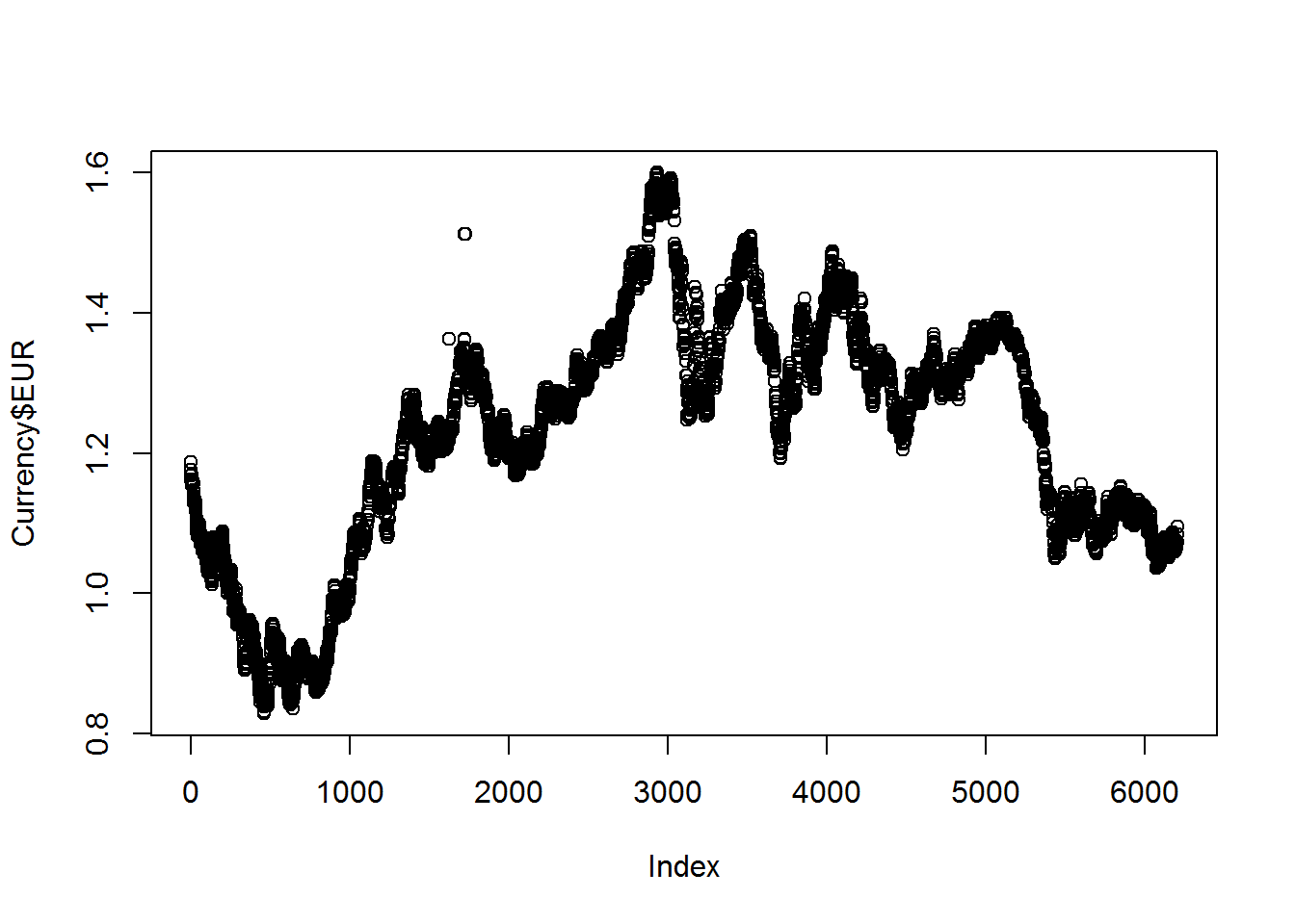
Hmm… it’s quite ugly… We will improve it later.
1.3.4. Read values from binary file
R can keep data in GZip-ed form, automatically loading the variables into memory. Such files have .RData extension. This is a fast & easy way to store your data. Let us first download the data in RData format into you working directory using download.file() and then load it by load(). Parameters of downloading:
destfile- the file name, under which you would like to store the downloaded file.mode- the way you would like to treat the data (as text or binary). To keep binary data unchanged, usewb!
download.file("http://edu.sablab.net/data/all.Rdata",
              destfile="all.Rdata",mode = "wb")

getwd()                # show current folder
dir(pattern=".Rdata")  # show files in the current folder
load("all.RData")      # load the data

ls()                   # you should see 'GE.matrix' among variables

View(GE.matrix)
You can see row and column names of the loaded data.frame object:
attr(GE.matrix,"dimnames")    # annotation of the dimensions
rownames(GE.matrix)
colnames(GE.matrix)
1.3.5. Data export
There are several ways to export your data. Let’s consider the most simple.
write()- writes a column of numbers / characterswrite.table()- writes a data tablesave()- saves one or several variables into a binary RData file.
Parameters of write.table are:
eol- cheracter for the end of line (can be differ with OS). The standard one is “”dec- decimal separatorquote- do we put “” around character values or notrow.names- do we put row names as a column or not
write.table(Currency,file = "curr.txt",sep = "\t",
            eol = "\n", na = "NA", dec = ".",
            row.names = FALSE, quote=FALSE)

save(Currency,file="Currency.Rdata") # save as binary file

save(list=ls(),file="workspace.Rdata") # save all variables as binary file

getwd()
dir()      # see the results
Exercises 1.3
- Dataset from http://edu.sablab.net/data/txt/shop.txt contains records about customers, collected by a women’s apparel store. Check its structure. View its summary.
read.table,View,str,summary,head
- For the “shop” table, save into a new text file only the records for customers, who paid using Visa card.
write.table
1.4. Workflow Control and Custom Functions
This section is optional. We consider here the conditional operators (if/else) and loops, which can be avoided working in R.
1.4.1. Conditions
a=1
b=2

if (a==b) {
  print("a equals to b")
} else {
  print("a is not equal to b")
}

## use if in-a-line
ifelse(a==b, "equal", "different")
1.4.2. Loops
Using loops in R is not recommended. You should avoid them, when possible, because of very slow execution. R is interpretable language, not precompiled (opposite to C).
FOR
Runs the same code for each values of the ‘iterator’.
# load some data
Shop = read.table("http://edu.sablab.net/data/txt/shop.txt",header=T,sep="\t")

# print all information for the first client
for (i in 1:ncol(Shop) ){
  print(Shop[1,i])
}
WHILE loop
Similar to FOR, but without iterator (we have to introduce it)
# print all information for the first client
i=1;
while (i <= ncol(Shop)){
  print(Shop[1,i])
  i=i+1
}
REPEAT loop
i=1
repeat {
  print(i)
  i=i+1
  if (i>10) break
}
Keywords break (stop loop) and next (switch to the next iteration) help to control the workflow.
1.4.3. Custom functions
Let us write own function to print vectors.
printVector = function(x, name=""){
  print(paste("Vector",name,"with",length(x),"elements:")) # print header
  if (length(x)>0) # if vector is not empty
    for (i in 1:length(x)) # for each element
      print(paste(name,"[",i,"] =",as.character(x[i]))) # print value
}

printVector(Shop$Payment, "Payment")
You can run scripts saved on a web page using source():
source("http://sablab.net/scripts/plotPCA.r")

plotPCA
Exercises 1.4 (optional)
These three tasks can be dome without using loops (by matrix operations). So, consider it only as an example.
- Create a matrix 8x8. Fill it with 0. Using “for” loop change elements of the main diagonal to 1.
matrix,for
##      [,1] [,2] [,3] [,4] [,5] [,6] [,7] [,8]
## [1,]    1    0    0    0    0    0    0    0
## [2,]    0    1    0    0    0    0    0    0
## [3,]    0    0    1    0    0    0    0    0
## [4,]    0    0    0    1    0    0    0    0
## [5,]    0    0    0    0    1    0    0    0
## [6,]    0    0    0    0    0    1    0    0
## [7,]    0    0    0    0    0    0    1    0
## [8,]    0    0    0    0    0    0    0    1
- Fill a matrix 8x8 with “1” to get a chess-board, where 0 codes a white cell and 1 - a black cell. Note, that black cells appear only if the sum of indexes is an even number (1+1=2, 1+3=4, 2+2=4, etc).
matrix,for,if
##      [,1] [,2] [,3] [,4] [,5] [,6] [,7] [,8]
## [1,]    1    0    1    0    1    0    1    0
## [2,]    0    1    0    1    0    1    0    1
## [3,]    1    0    1    0    1    0    1    0
## [4,]    0    1    0    1    0    1    0    1
## [5,]    1    0    1    0    1    0    1    0
## [6,]    0    1    0    1    0    1    0    1
## [7,]    1    0    1    0    1    0    1    0
## [8,]    0    1    0    1    0    1    0    1
- Calculate the sum of the first n=1000 members of the series:
s = (4/1) - (4/3) + (4/5) - (4/7) + (4/9) - (4/11) + (4/13) - (4/15) + ...Can you guess the value when n->Inf ?
1.5. Data Visualization
1.5.1. Plot time series
Let us come back to Currency dataset and improve the quality of its visualization.
Currency = read.table("http://edu.sablab.net/data/txt/currency.txt",header=T,as.is=T)First, we can initialize graphical window using x11().
- You can draw your image directly to the figure file using special devices:
pdf(),png(),tiff(),jpeg(). Always finalize drawing to file by callingdev.off()function (no parameters needed).
Please run line-by-line:
x11()  # try x11(width=8, height=5)

plot(Currency$EUR, pch=19, col = "blue", cex=2)

# pre-defined colors in R
colors()

# custom transparent color in #RRGGBB format:
plot(Currency$EUR, pch=19, col = "#00FF0033", cex=2)
There are many graphical parameters which you can tweak using par() functions. Please, have a look by ?par
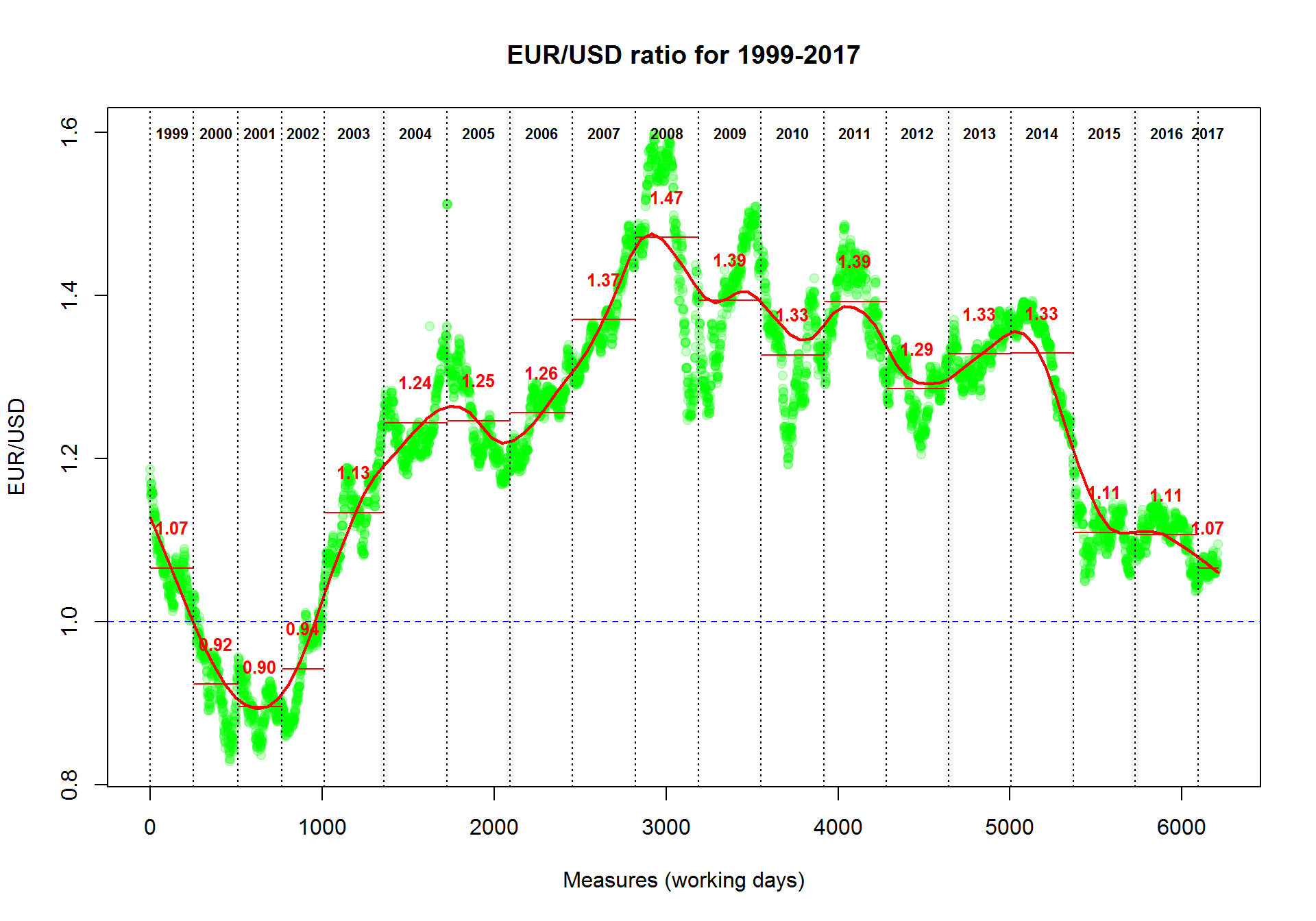
Now we will produce a more plot with smoothed interpolation and average rate for each year. We will add lines to existing plot using lines() and abline() functions. text() will write some text on the plot.
pch- dot shape code. Can be set to character, like"a"cex- size of the dotsmain- titlexlab,ylab- axis nameslwd- line thicknesslty- line type (solid, dashed, etc)font- normal=1, bold=2, etc
plot(Currency$EUR,col="#00FF0033",pch=19,
     main="EUR/USD ratio for 1999-2017",
     ylab="EUR/USD",
     xlab="Measures (working days)")

## add smoothing. Try different "f"
smooth = lowess(Currency$EUR,f=0.1)
lines(smooth,col="red",lwd=2)
## add 1 level
abline(h=1,col="blue",lty=2)

## (*) add years
year=1999  # an initial year
while (year<=2017){  # loop for all the years up to now
  # take the indexes of the measures for the "year"
  idx=grep(paste("^",year,sep=""),Currency$Date)
  # calculate the average ratio for the "year"
  average=mean(Currency$EUR[idx])
  # draw the year separator
  abline(v=min(idx),col=1,lty=3)
  # draw the average ratio for the "year"
  lines(x=c(min(idx),max(idx)),y=c(average,average),col=2)
  # write the years
  text(median(idx),max(Currency$EUR),sprintf("%d",year),font=2,cex=0.7)
  # write the average ratio
  text(median(idx),average+0.05,sprintf("%.2f",average),col=2,font=2,cex=0.8)
  year=year+1;
}
1.5.2. Visualize categorical data
Here we will work with a dataset from Mouse Phenome project. ‘Tordoff3’ dataset was downloaded and prepared for the analysis. See the file here: http://edu.sablab.net/data/txt/mice.txt
Let’s first load the data.
Mice = read.table("http://edu.sablab.net/data/txt/mice.txt", header=T, sep="\t")
str(Mice)
## 'data.frame': 790 obs. of 14 variables:
## $ ID : int 1 2 3 368 369 370 371 372 4 5 ...
## $ Strain : Factor w/ 40 levels "129S1/SvImJ",..: 1 1 1 1 1 1 1 1 1 1 ...
## $ Sex : Factor w/ 2 levels "f","m": 1 1 1 1 1 1 1 1 1 1 ...
## $ Starting.age : int 66 66 66 72 72 72 72 72 66 66 ...
## $ Ending.age : int 116 116 108 114 115 116 119 122 109 112 ...
## $ Starting.weight : num 19.3 19.1 17.9 18.3 20.2 18.8 19.4 18.3 17.2 19.7 ...
## $ Ending.weight : num 20.5 20.8 19.8 21 21.9 22.1 21.3 20.1 18.9 21.3 ...
## $ Weight.change : num 1.06 1.09 1.11 1.15 1.08 ...
## $ Bleeding.time : int 64 78 90 65 55 NA 49 73 41 129 ...
## $ Ionized.Ca.in.blood : num 1.2 1.15 1.16 1.26 1.23 1.21 1.24 1.17 1.25 1.14 ...
## $ Blood.pH : num 7.24 7.27 7.26 7.22 7.3 7.28 7.24 7.19 7.29 7.22 ...
## $ Bone.mineral.density: num 0.0605 0.0553 0.0546 0.0599 0.0623 0.0626 0.0632 0.0592 0.0513 0.0501 ...
## $ Lean.tissues.weight : num 14.5 13.9 13.8 15.4 15.6 16.4 16.6 16 14 16.3 ...
## $ Fat.weight : num 4.4 4.4 2.9 4.2 4.3 4.3 5.4 4.1 3.2 5.2 ...If you would like to have an overview of the data, and you have a reasonable number of columns, you can just plot() all possible scatter plots for your data.frame
plot(Mice, pch=".", col="blue")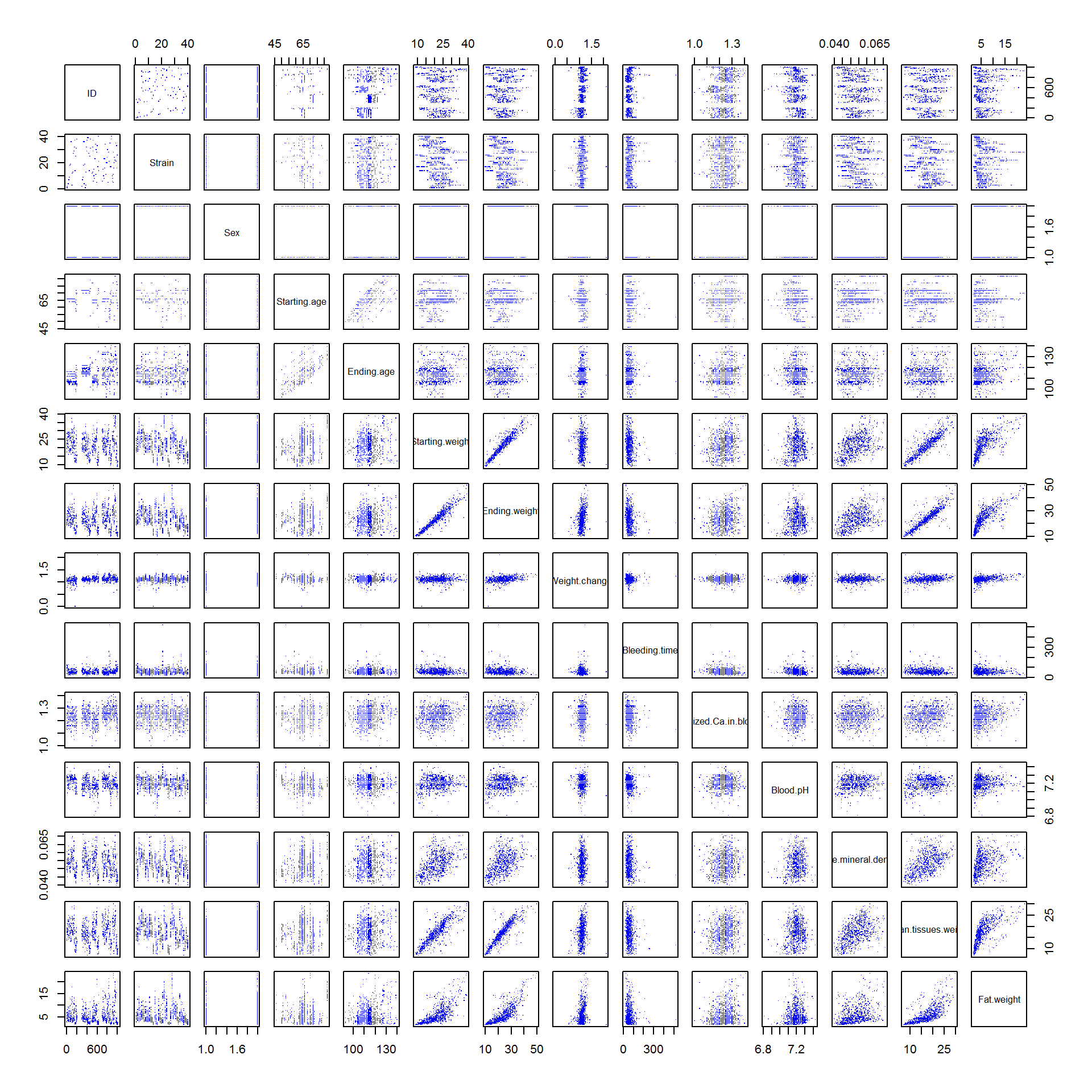
Let us plot some factorial data. For example, we can check how well was the experiment designed with respect to mouse strain.
plot(Mice$Strain)Or do it more beautifully:
las- axis text direction (2 for perpendicular)cex.names- size of the category names on the horizontal axis
plot(Mice$Strain, las=2, col=rainbow(nlevels(Mice$Strain)), cex.names =0.7)
title("Number of mice from each strain")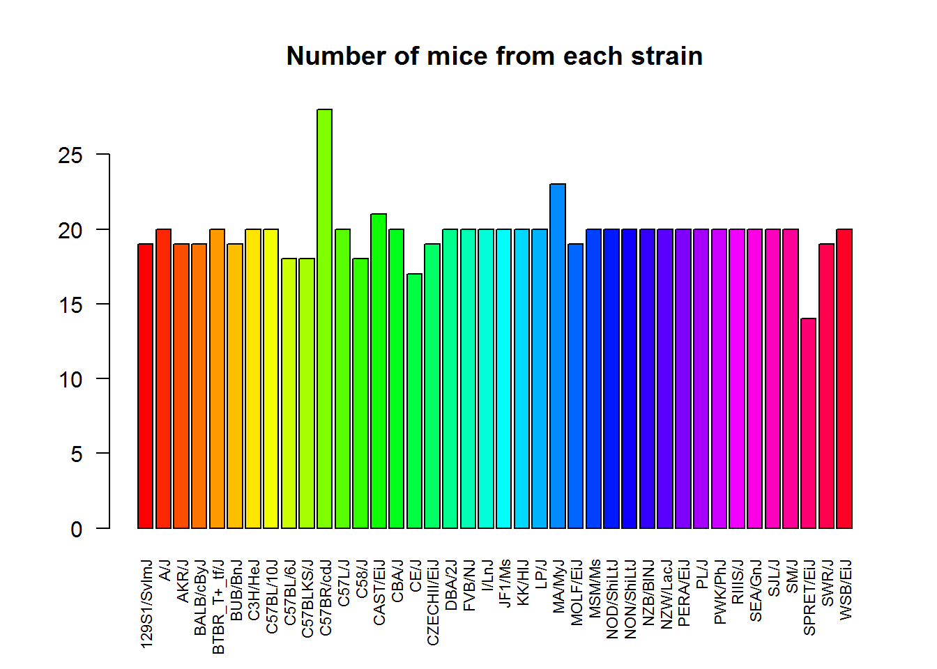
Pie-chart
pie(summary(Mice$Sex), col=c("pink","lightblue"))
title("Gender composition (f:female, m:male)")
5.3. Distributions and box-plot
Distributions can be shown using hist() or plot(density()) functions.
hist(Mice$Starting.weight,probability = T, main="Histogram and p.d.f. approximation", xlab="weight, g")
lines(density(Mice$Starting.weight),lwd=2,col=4)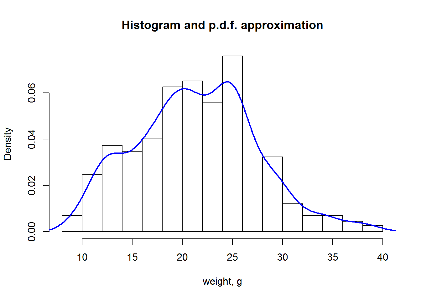
Now let us build a standard boxplot that shows starting weight for male and female mice. We will use formula here: ‘variable’ ~ ‘factor’. It is the easiest way.
boxplot(Starting.weight ~ Sex, data=Mice, col=c("pink","lightblue"))
title("Weight by sex (f:female,b m:male)",  ylab="weight, g",xlab="sex")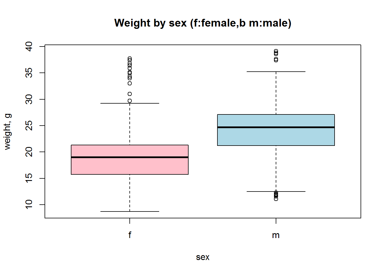
5.4. Heatmaps
Heatmaps are a useful 2D representation of the data that have 3 dimensions. Example: expression (dim 1) is measured over n genes (dim 2) in m samples (dim 3). Heatmaps will automatically cluster the data (see Lecture 9). Let us make a heatmap for internal Iris dataset. We should also transform data.frame to a matrix
# see iris dataset
str(iris)

# let us transform the data to a matrix
X = as.matrix(iris[,-5])
heatmap(t(X))
``
# add species as colors
color = as.integer(iris[,5])
str(color)
## int [1:150] 1 1 1 1 1 1 1 1 1 1 ...color = rainbow(4)[color]
str(color)## chr [1:150] "#FF0000FF" "#FF0000FF" "#FF0000FF" "#FF0000FF" ...heatmap(t(X),ColSideColors = color)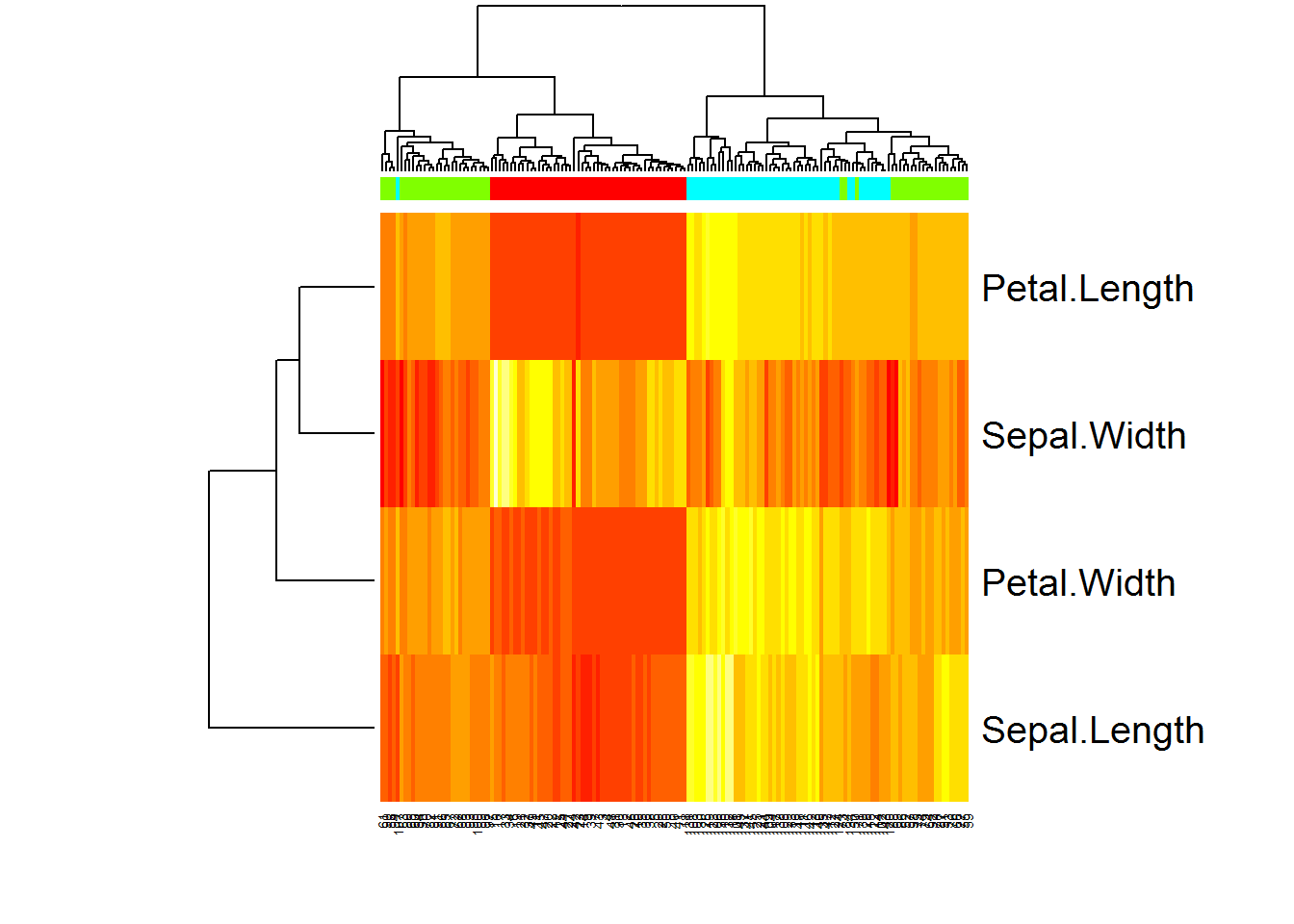
More advanced heatmaps can be built using pheatmap package.
5.5. 3D visualization
There are options for 3D plotting in R. See static images in demo(persp) And here is an interactiv 3D plot using rgl package:
library(rgl)

# define coordinates
x=Mice$Starting.weight
y=Mice$Ending.weight
z=Mice$Fat.weight

# plot in 3D
plot3d(x,y,z)
Exercises 1.5
- Use mice dataset. Build distributions for male and female body weights in one plot.
plot,density
- Draw boxplots, showing variability of bleeding time for mice of different strains.
boxplot
![]()