- Basic Statistics
Petr V. Nazarov, LIH
2017-05-29 / 2017-05-30
Let’s load again Mice data:
## clear memory
rm(list = ls())
## load data
Mice=read.table("http://edu.sablab.net/data/txt/mice.txt",header=T,sep="\t")
str(Mice)
## 'data.frame': 790 obs. of 14 variables:
## $ ID : int 1 2 3 368 369 370 371 372 4 5 ...
## $ Strain : Factor w/ 40 levels "129S1/SvImJ",..: 1 1 1 1 1 1 1 1 1 1 ...
## $ Sex : Factor w/ 2 levels "f","m": 1 1 1 1 1 1 1 1 1 1 ...
## $ Starting.age : int 66 66 66 72 72 72 72 72 66 66 ...
## $ Ending.age : int 116 116 108 114 115 116 119 122 109 112 ...
## $ Starting.weight : num 19.3 19.1 17.9 18.3 20.2 18.8 19.4 18.3 17.2 19.7 ...
## $ Ending.weight : num 20.5 20.8 19.8 21 21.9 22.1 21.3 20.1 18.9 21.3 ...
## $ Weight.change : num 1.06 1.09 1.11 1.15 1.08 ...
## $ Bleeding.time : int 64 78 90 65 55 NA 49 73 41 129 ...
## $ Ionized.Ca.in.blood : num 1.2 1.15 1.16 1.26 1.23 1.21 1.24 1.17 1.25 1.14 ...
## $ Blood.pH : num 7.24 7.27 7.26 7.22 7.3 7.28 7.24 7.19 7.29 7.22 ...
## $ Bone.mineral.density: num 0.0605 0.0553 0.0546 0.0599 0.0623 0.0626 0.0632 0.0592 0.0513 0.0501 ...
## $ Lean.tissues.weight : num 14.5 13.9 13.8 15.4 15.6 16.4 16.6 16 14 16.3 ...
## $ Fat.weight : num 4.4 4.4 2.9 4.2 4.3 4.3 5.4 4.1 3.2 5.2 ...2.1. Desctiptive Statistics
2.1.1. Measures of the center
summary(Mice)## ID Strain Sex Starting.age
## Min. : 1.0 C57BR/cdJ : 28 f:396 Min. :46.00
## 1st Qu.: 310.2 MA/MyJ : 23 m:394 1st Qu.:64.00
## Median : 537.5 CAST/EiJ : 21 Median :66.00
## Mean : 526.8 A/J : 20 Mean :66.21
## 3rd Qu.: 799.8 BTBR_T+_tf/J: 20 3rd Qu.:71.00
## Max. :1012.0 C3H/HeJ : 20 Max. :82.00
## (Other) :658
## Ending.age Starting.weight Ending.weight Weight.change
## Min. : 93.0 Min. : 8.70 Min. :10.00 Min. :0.000
## 1st Qu.:109.0 1st Qu.:17.20 1st Qu.:18.80 1st Qu.:1.059
## Median :114.0 Median :21.20 Median :23.50 Median :1.105
## Mean :114.3 Mean :21.38 Mean :23.69 Mean :1.107
## 3rd Qu.:119.0 3rd Qu.:25.38 3rd Qu.:28.10 3rd Qu.:1.164
## Max. :140.0 Max. :39.10 Max. :49.60 Max. :2.109
## NA's :2
## Bleeding.time Ionized.Ca.in.blood Blood.pH Bone.mineral.density
## Min. : 14 Min. :1.000 Min. :6.810 Min. :0.03980
## 1st Qu.: 43 1st Qu.:1.200 1st Qu.:7.160 1st Qu.:0.04860
## Median : 55 Median :1.240 Median :7.200 Median :0.05300
## Mean : 61 Mean :1.237 Mean :7.199 Mean :0.05331
## 3rd Qu.: 73 3rd Qu.:1.280 3rd Qu.:7.250 3rd Qu.:0.05785
## Max. :522 Max. :1.410 Max. :7.430 Max. :0.07140
## NA's :30 NA's :2 NA's :2 NA's :3
## Lean.tissues.weight Fat.weight
## Min. : 7.30 Min. : 1.800
## 1st Qu.:13.80 1st Qu.: 3.500
## Median :17.30 Median : 4.800
## Mean :17.27 Mean : 6.073
## 3rd Qu.:20.85 3rd Qu.: 7.500
## Max. :29.90 Max. :23.300
## NA's :3 NA's :3## mean and median. We should exclude NA from consideration
mn = mean(Mice$Ending.weight, na.rm=T)
md = median(Mice$Ending.weight, na.rm=T)
## for mode you should add a library:
library(modeest)##
## This is package 'modeest' written by P. PONCET.
## For a complete list of functions, use 'library(help = "modeest")' or 'help.start()'.mo = mlv(Mice$Ending.weight, method = "shorth")$M
## let us plot them
plot(density(Mice$Ending.weight, na.rm=T),lwd=2,main="Ending weight")
abline(v = mn,col="red")
abline(v = md,col="blue")
abline(v = mo ,col="cyan")
legend(x="topright",c("mean","median","mode"),col=c("red","blue","cyan"),pch=19)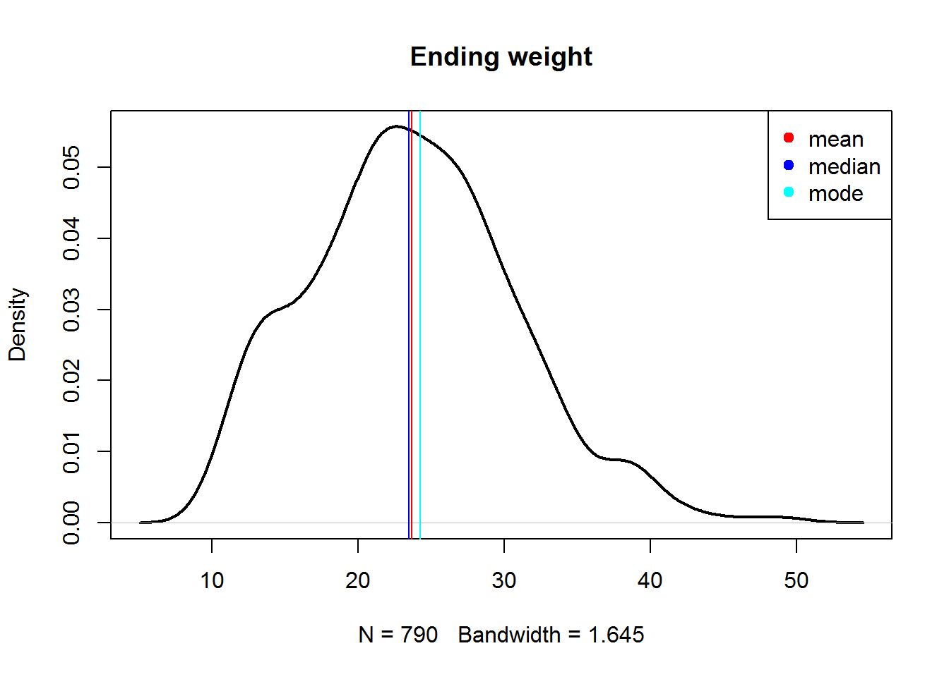
2.1.2. Measures of variation
## quantiles, percentiles and quartiles
quantile(Mice$Bleeding.time,prob=c(0.25,0.5,0.75),na.rm=T)
## 25% 50% 75%
## 43 55 73## standard deviation and variance
sd(Mice$Bleeding.time, na.rm=T)## [1] 31.91943var(Mice$Bleeding.time, na.rm=T)## [1] 1018.85## stable measure of variation - MAD
mad(Mice$Bleeding.time, na.rm=T)## [1] 20.7564mad(Mice$Bleeding.time, constant = 1, na.rm=T)## [1] 142.1.3. Measures of dependency
## covariation
cov(Mice$Starting.weight,Mice$Ending.weight)
## [1] 39.84946## correlation
cor(Mice$Starting.weight,Mice$Ending.weight)## [1] 0.9422581## coefficient of determination, R2
cor(Mice$Starting.weight,Mice$Ending.weight)^2## [1] 0.8878503## kendal correlation
cor(Mice$Starting.weight,Mice$Ending.weight,method="kendal")## [1] 0.8188964## spearman correlation
cor(Mice$Starting.weight,Mice$Ending.weight,method="spearman")## [1] 0.9423666Excercises 2.1.
- Use mice dataset. Calculate the number of mice with bleeding time bigger than 2 minutes
read.table,sum
- Report a 5-numer summary for each column of “mice” data
summary
- For dataset “mice” replace starting weight of any mouse by 1000 (assume, there is a mistype). Calculate mean, median, standard deviation and median absolute deviation (MAD) of this weight. Compare the results with original measures.
mean,median,sd,mad
2.2. Statistical Tests
2.2.1. Hypotheses about mean of a population
| \[ \begin{align} H_0 : \mu \le \mu_0 \\ H_1 : \mu > \mu_0 \end{align} \] | \[ \begin{align} H_0 : \mu \ge \mu_0 \\ H_1 : \mu < \mu_0 \end{align} \] | \[ \begin{align} H_0 : \mu = \mu_0 \\ H_1 : \mu \ne \mu_0 \end{align} \] |
Let’s consider the following example. The number of living cells in 5 wells under some conditions are given below. In a reference literature source authors claimed a mean quantity of 5000 living cells under the same conditions. Is our result significantly different?
x =c(5128,4806,5037,4231,4222)

# one sample t-test
t.test(x,mu=5000)
##
## One Sample t-test
##
## data: x
## t = -1.622, df = 4, p-value = 0.1801
## alternative hypothesis: true mean is not equal to 5000
## 95 percent confidence interval:
## 4145.255 5224.345
## sample estimates:
## mean of x
## 4684.82.2.2. Hypotheses about mean of a population
| \[ \begin{align} H_0 : \pi \le \pi_0 \\ H_1 : \pi > \pi_0 \end{align} \] | \[ \begin{align} H_0 : \pi \ge \pi_0 \\ H_1 : \pi < \pi_0 \end{align} \] | \[ \begin{align} H_0 : \pi = \pi_0 \\ H_1 : \pi \ne \pi_0 \end{align} \] |
R can help testing hypotheses about proportions.
Example: During a study of a new drug against viral infection, you have found that 70 out of 100 mice survived, whereas the survival after the standard therapy is 60% of the infected population. Is this enhancement statistically significant?
## make analysis by prop.test(). Approximate!
prop.test(x=70,n=100,p=0.6,alternative="greater")
##
## 1-sample proportions test with continuity correction
##
## data: 70 out of 100, null probability 0.6
## X-squared = 3.7604, df = 1, p-value = 0.02624
## alternative hypothesis: true p is greater than 0.6
## 95 percent confidence interval:
## 0.6149607 1.0000000
## sample estimates:
## p
## 0.7## make analysis by binom.test(). Exact!
binom.test(x=70,n=100,p=0.6,alternative="greater")##
## Exact binomial test
##
## data: 70 and 100
## number of successes = 70, number of trials = 100, p-value =
## 0.02478
## alternative hypothesis: true probability of success is greater than 0.6
## 95 percent confidence interval:
## 0.6157794 1.0000000
## sample estimates:
## probability of success
## 0.72.2.3. Comparing means of 2 unmatched samples
| \[ \begin{align} H_0 : \mu_1 \le \mu_2 \\ H_1 : \mu_1 > \mu_2 \end{align} \] | \[ \begin{align} H_0 : \mu_1 \ge \mu_2 \\ H_1 : \mu_1 < \mu_2 \end{align} \] | \[ \begin{align} H_0 : \mu_1 = \mu_2 \\ H_1 : \mu_1 \ne \mu_2 \end{align} \] |
Parametric version of this comparison is done unig t.test(). Non-parametric - wilcox.test().
Mice=read.table("http://edu.sablab.net/data/txt/mice.txt",header=T,sep="\t")

# ending weight for male and female
xm = Mice$Ending.weight[Mice$Sex=="m"]
xf = Mice$Ending.weight[Mice$Sex=="f"]
t.test(xm,xf)
##
## Welch Two Sample t-test
##
## data: xm and xf
## t = 13.582, df = 759.53, p-value < 2.2e-16
## alternative hypothesis: true difference in means is not equal to 0
## 95 percent confidence interval:
## 5.265756 7.045119
## sample estimates:
## mean of x mean of y
## 26.77665 20.62121wilcox.test(xm,xf)##
## Wilcoxon rank sum test with continuity correction
##
## data: xm and xf
## W = 120510, p-value < 2.2e-16
## alternative hypothesis: true location shift is not equal to 0# weight change for male & female
xm = Mice$Weight.change[Mice$Sex=="m"]
xf = Mice$Weight.change[Mice$Sex=="f"]
t.test(xm,xf)##
## Welch Two Sample t-test
##
## data: xm and xf
## t = 3.2067, df = 682.86, p-value = 0.001405
## alternative hypothesis: true difference in means is not equal to 0
## 95 percent confidence interval:
## 0.009873477 0.041059866
## sample estimates:
## mean of x mean of y
## 1.119401 1.093934wilcox.test(xm,xf)##
## Wilcoxon rank sum test with continuity correction
##
## data: xm and xf
## W = 84976, p-value = 0.02989
## alternative hypothesis: true location shift is not equal to 0# bleeding time male & female
xm = Mice$Bleeding.time[Mice$Sex=="m"]
xf = Mice$Bleeding.time[Mice$Sex=="f"]
t.test(xm,xf)##
## Welch Two Sample t-test
##
## data: xm and xf
## t = -1.1544, df = 722.78, p-value = 0.2487
## alternative hypothesis: true difference in means is not equal to 0
## 95 percent confidence interval:
## -7.213644 1.871515
## sample estimates:
## mean of x mean of y
## 59.66667 62.33773wilcox.test(xm,xf)##
## Wilcoxon rank sum test with continuity correction
##
## data: xm and xf
## W = 65030, p-value = 0.01781
## alternative hypothesis: true location shift is not equal to 02.2.4. Matched samples
Example. The systolic blood pressures of n=12 women between the ages of 20 and 35 were measured before and after usage of a newly developed oral contraceptive.
BP=read.table("http://edu.sablab.net/data/txt/bloodpressure.txt",header=T,sep="\t")
str(BP)
## 'data.frame': 12 obs. of 3 variables:
## $ Subject : int 1 2 3 4 5 6 7 8 9 10 ...
## $ BP.before: int 122 126 132 120 142 130 142 137 128 132 ...
## $ BP.after : int 127 128 140 119 145 130 148 135 129 137 ...## Unpaired
t.test(BP$BP.before,BP$BP.after)##
## Welch Two Sample t-test
##
## data: BP$BP.before and BP$BP.after
## t = -0.83189, df = 21.387, p-value = 0.4147
## alternative hypothesis: true difference in means is not equal to 0
## 95 percent confidence interval:
## -9.034199 3.867532
## sample estimates:
## mean of x mean of y
## 130.6667 133.2500wilcox.test(BP$BP.before,BP$BP.after)## Warning in wilcox.test.default(BP$BP.before, BP$BP.after): cannot compute
## exact p-value with ties##
## Wilcoxon rank sum test with continuity correction
##
## data: BP$BP.before and BP$BP.after
## W = 59.5, p-value = 0.487
## alternative hypothesis: true location shift is not equal to 0## Paired
t.test(BP$BP.before,BP$BP.after,paired=T)##
## Paired t-test
##
## data: BP$BP.before and BP$BP.after
## t = -2.8976, df = 11, p-value = 0.01451
## alternative hypothesis: true difference in means is not equal to 0
## 95 percent confidence interval:
## -4.5455745 -0.6210921
## sample estimates:
## mean of the differences
## -2.583333wilcox.test(BP$BP.before,BP$BP.after,paired=T)## Warning in wilcox.test.default(BP$BP.before, BP$BP.after, paired = T):
## cannot compute exact p-value with ties## Warning in wilcox.test.default(BP$BP.before, BP$BP.after, paired = T):
## cannot compute exact p-value with zeroes##
## Wilcoxon signed rank test with continuity correction
##
## data: BP$BP.before and BP$BP.after
## V = 5, p-value = 0.02465
## alternative hypothesis: true location shift is not equal to 02.2.5. Comparing proportions in two populations
| \[ \begin{align} H_0 : \pi_1 \le \pi_2 \\ H_1 : \pi_1 > \pi_2 \end{align} \] | \[ \begin{align} H_0 : \pi_1 \ge \pi_2 \\ H_1 : \pi_1 < \pi_2 \end{align} \] | \[ \begin{align} H_0 : \pi_1 = \pi_2 \\ H_1 : \pi_1 \ne \pi_2 \end{align} \] |
x = Mice$Sex[Mice$Strain == "SWR/J"]
y = Mice$Sex[Mice$Strain == "MA/MyJ"]
prop.test(c(sum(x=="m"),sum(y=="m")),n=c(length(x),length(y)))
##
## 2-sample test for equality of proportions with continuity
## correction
##
## data: c(sum(x == "m"), sum(y == "m")) out of c(length(x), length(y))
## X-squared = 0.72283, df = 1, p-value = 0.3952
## alternative hypothesis: two.sided
## 95 percent confidence interval:
## -0.5236857 0.1667063
## sample estimates:
## prop 1 prop 2
## 0.4736842 0.65217392.2.6. Comparing variances of two populations
| \[ \begin{align} H_0 : \sigma^2_1 = \sigma^2_2 \\ H_1 : \sigma^2_1 \ne \sigma^2_2 \end{align} \] |
Example. A school is selecting a company to probide school bus to its pupils. They would like to choose the most punctual one. The times between bus arrival of wto companies were measured and stored in schoolbus dataset. Please test whether the difference is significant with \(\alpha = 0.1\).
Bus=read.table("http://edu.sablab.net/data/txt/schoolbus.txt",header=T,sep="\t")
str(Bus)
## 'data.frame': 26 obs. of 2 variables:
## $ Milbank : num 35.9 29.9 31.2 16.2 19 15.9 18.8 22.2 19.9 16.4 ...
## $ Gulf.Park: num 21.6 20.5 23.3 18.8 17.2 7.7 18.6 18.7 20.4 22.4 ...var.test(Bus[,1], Bus[,2])##
## F test to compare two variances
##
## data: Bus[, 1] and Bus[, 2]
## F = 2.401, num df = 25, denom df = 15, p-value = 0.08105
## alternative hypothesis: true ratio of variances is not equal to 1
## 95 percent confidence interval:
## 0.8927789 5.7887880
## sample estimates:
## ratio of variances
## 2.4010362.2.7. Significance of correlation
Example. A malacologist interested in the morphology of West Indian chitons, Chiton olivaceous, measured the length and width of the eight overlapping plates composing the shell of 10 of these animals.
Chiton =read.table("http://edu.sablab.net/data/txt/chiton.txt",header=T,sep="\t")
str(Chiton)
## 'data.frame': 10 obs. of 2 variables:
## $ Length: num 10.7 11 9.5 11.1 10.3 10.7 9.9 10.6 10 12
## $ Width : num 5.8 6 5 6 5.3 5.8 5.2 5.7 5.3 6.3plot(Chiton,pch=19,main=sprintf("r = %.4f",cor(Chiton[,1],Chiton[,2])))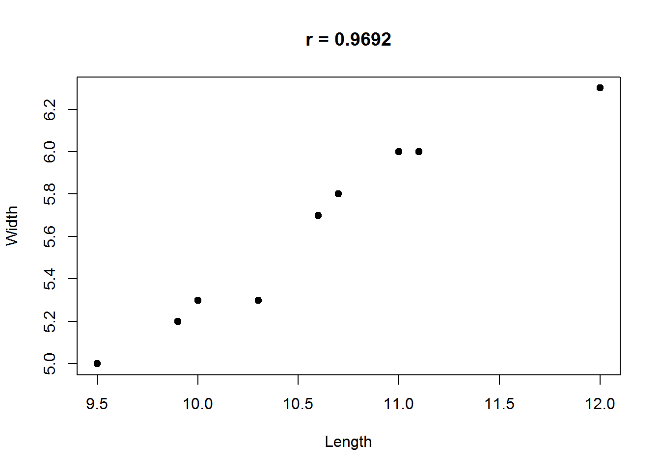
cor.test(Chiton$Length,Chiton$Width)##
## Pearson's product-moment correlation
##
## data: Chiton$Length and Chiton$Width
## t = 11.136, df = 8, p-value = 3.781e-06
## alternative hypothesis: true correlation is not equal to 0
## 95 percent confidence interval:
## 0.8713272 0.9929217
## sample estimates:
## cor
## 0.969226Exercises 2.2
- See
gliodataset. Assume, that an average survival time for glioblastoma patients (early state, age<50) is 18 months. You developed a new treatment, which should increase the survival time and performed a pilot clinical trial (10 patients) in order to determine the positive effect. Is the survival improve significant?
- Based on complete
micedata set, means of which parameters (except weight) are significantly different for male and female populations?
- Look for dataset
cancerThis data contains results of survey aimed at survival and life quality of patients with advanced lung cancer, performed by the North Central Cancer Treatment Group (Loprinzi CL et al, J. of Clinical Oncology. 12(3):601-7, 1994). Look for the survival time (column time, given in days) and compare the survival for male and female populations . Apply both parametric and non-parametric testing. What happent if you log-transform the data?
- See
leukemiaThis dataset contains information about two groups of patients who died of acute myelogenous leukemia. Patients were classified into the two groups according to the presence or absence of a morphologic characteristic of white cells. Patients termed AG positive were identified by the presence of Auer rods and/or significant granulature of the leukemic cells in the bone marrow at diagnosis. For AG-negative patients, these factors were absent. Leukemia is a cancer characterized by an overproliferation of white blood cells; the higher the white blood count (WBC), the more severe the disease. Investigate the data using parametric and non-parametric tests.
2.3. Detection of outliers
Let’s consider several methods to detect outliers
## load data
Mice=read.table("http://edu.sablab.net/data/txt/mice.txt", header=T,sep="\t")
x=Mice$Weight.change
2.3.1 Simple z-score
z = scale(x)
plot(abs(z),pch=19,col="blue",main="|z|")
abline(h=3,col=2)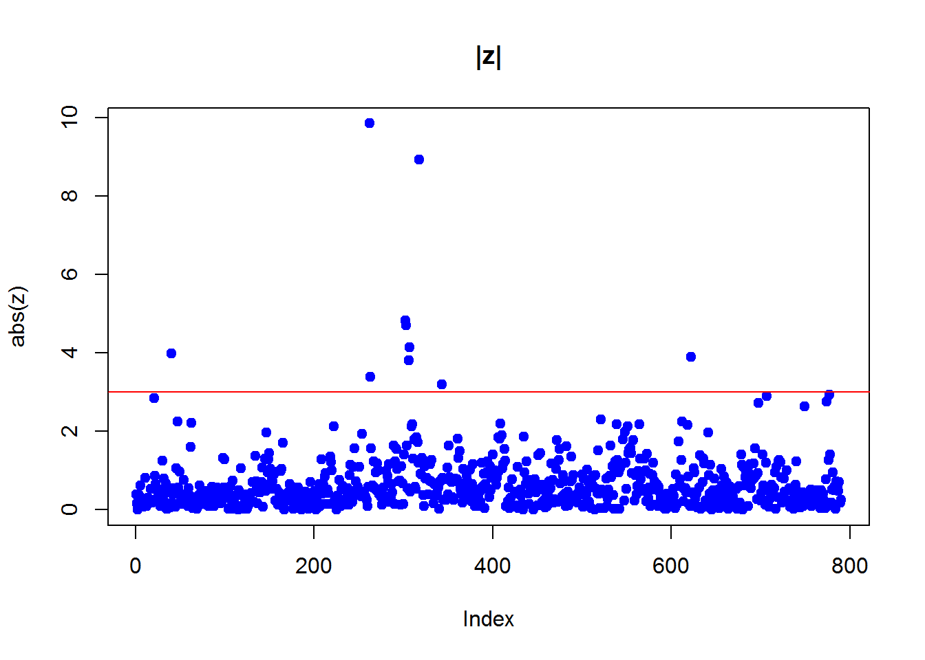
2.3.2 Iglewicz-Hoaglin method
z = (x-median(x)) / mad(x)
plot(abs(z),pch=19,col=4,main="|z| by Iglewicz-Hoaglin")
abline(h=3.5,col=2)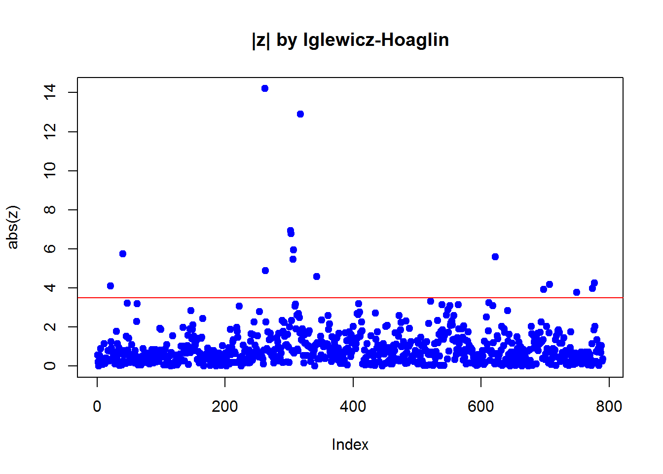
2.3.3. Grubb’s method
library(outliers)
x1=x
while(grubbs.test(x1)$p.value < 0.05){
  x1[x1==outlier(x1)]=NA
}
plot(abs(x-mean(x1,na.rm=T))/sd(x1,na.rm=T),pch=19,col="red",main="Outliers by Grubb's Test")
points(abs(x1-mean(x1,na.rm=T))/sd(x1,na.rm=T),pch=19,col="blue")
![]()