- Linear Models
Petr V. Nazarov, LIH
2017-05-30
3.1. ANOVA - analysis of variance
Please see lecture 3.1 for explanations about ANOVA.
As part of a long-term study of individuals 65 years of age or older, sociologists and physicians at the Wentworth Medical Center in upstate New York investigated the relationship between geographic location and depression. A sample of 60 individuals, all in reasonably good health, and 60 in bad health was selected; 20 individuals were residents of Florida, 20 were residents of New York, and 20 were residents of North Carolina. Each of the individuals sampled was given a standardized test to measure depression. The data collected follow; higher test scores indicate higher levels of depression.
## load data
Data = read.table("http://edu.sablab.net/data/txt/depression2.txt",header=T,sep="\t")
str(Data)
## 'data.frame': 120 obs. of 3 variables:
## $ Location : Factor w/ 3 levels "Florida","New York",..: 1 1 1 1 1 1 1 1 1 1 ...
## $ Health : Factor w/ 2 levels "bad","good": 2 2 2 2 2 2 2 2 2 2 ...
## $ Depression: int 3 7 7 3 8 8 8 5 5 2 ...3.1.1. One-way ANOVA
Let’s take good health people first and see the effect of the location.
DataGH = Data[Data$Health == "good",]

## build 1-factor ANOVA model
res1 = aov(Depression ~  Location, DataGH)
summary(res1)
## Df Sum Sq Mean Sq F value Pr(>F)
## Location 2 78.5 39.27 6.773 0.0023 **
## Residuals 57 330.4 5.80
## ---
## Signif. codes: 0 '***' 0.001 '**' 0.01 '*' 0.05 '.' 0.1 ' ' 13.1.2. Two-way ANOVA
Now, let’s use all data, including bad health respondents.
res2 = aov(Depression ~  Location + Health + Location*Health, data = Data)

## show the ANOVA table
summary(res2)
## Df Sum Sq Mean Sq F value Pr(>F)
## Location 2 73.8 36.9 4.290 0.016 *
## Health 1 1748.0 1748.0 203.094 <2e-16 ***
## Location:Health 2 26.1 13.1 1.517 0.224
## Residuals 114 981.2 8.6
## ---
## Signif. codes: 0 '***' 0.001 '**' 0.01 '*' 0.05 '.' 0.1 ' ' 1We can remove interactions (assume that the effects are purely additive)
res2ni = aov(Depression ~  Location + Health, data = Data)
summary(res2ni)
## Df Sum Sq Mean Sq F value Pr(>F)
## Location 2 73.8 36.9 4.252 0.0165 *
## Health 1 1748.0 1748.0 201.299 <2e-16 ***
## Residuals 116 1007.3 8.7
## ---
## Signif. codes: 0 '***' 0.001 '**' 0.01 '*' 0.05 '.' 0.1 ' ' 1Some examples of reporting the importance:
## get p-values
pv=(summary(res2)[[1]][,5])
names(pv) = rownames(summary(res2)[[1]])
barplot(-log(pv),ylab="-log10(p-value)")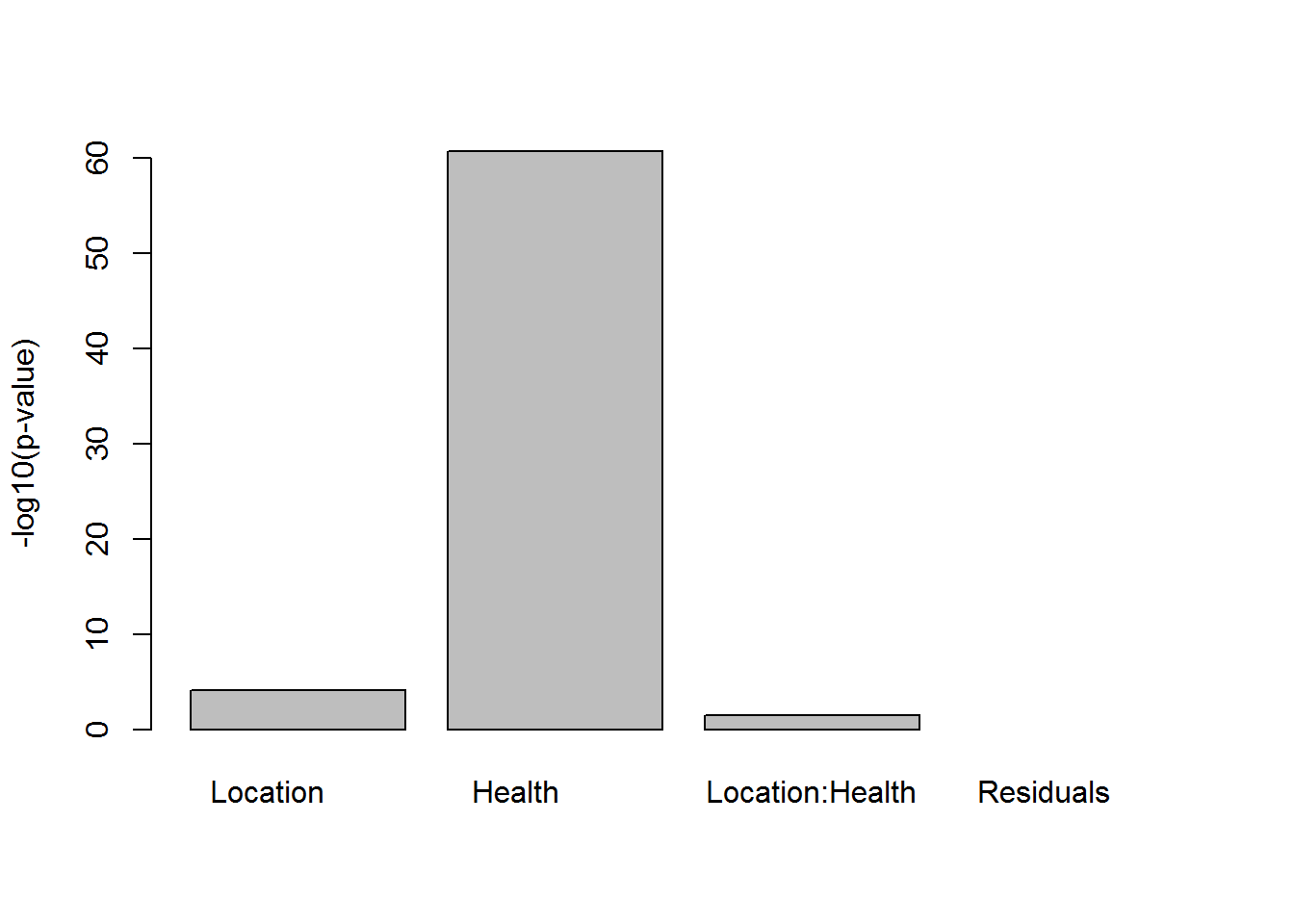
3.1.3. Post-hoc analysis
TukeyHSD(res1)## Tukey multiple comparisons of means
## 95% family-wise confidence level
##
## Fit: aov(formula = Depression ~ Location, data = DataGH)
##
## $Location
## diff lwr upr p adj
## New York-Florida 2.8 0.9677423 4.6322577 0.0014973
## North Carolina-Florida 1.5 -0.3322577 3.3322577 0.1289579
## North Carolina-New York -1.3 -3.1322577 0.5322577 0.2112612TukeyHSD(res2)## Tukey multiple comparisons of means
## 95% family-wise confidence level
##
## Fit: aov(formula = Depression ~ Location + Health + Location * Health, data = Data)
##
## $Location
## diff lwr upr p adj
## New York-Florida 1.850 0.2921599 3.4078401 0.0155179
## North Carolina-Florida 0.475 -1.0828401 2.0328401 0.7497611
## North Carolina-New York -1.375 -2.9328401 0.1828401 0.0951631
##
## $Health
## diff lwr upr p adj
## good-bad -7.633333 -8.694414 -6.572252 0
##
## $`Location:Health`
## diff lwr upr
## New York:bad-Florida:bad 0.90 -1.7893115 3.589311
## North Carolina:bad-Florida:bad -0.55 -3.2393115 2.139311
## Florida:good-Florida:bad -8.95 -11.6393115 -6.260689
## New York:good-Florida:bad -6.15 -8.8393115 -3.460689
## North Carolina:good-Florida:bad -7.45 -10.1393115 -4.760689
## North Carolina:bad-New York:bad -1.45 -4.1393115 1.239311
## Florida:good-New York:bad -9.85 -12.5393115 -7.160689
## New York:good-New York:bad -7.05 -9.7393115 -4.360689
## North Carolina:good-New York:bad -8.35 -11.0393115 -5.660689
## Florida:good-North Carolina:bad -8.40 -11.0893115 -5.710689
## New York:good-North Carolina:bad -5.60 -8.2893115 -2.910689
## North Carolina:good-North Carolina:bad -6.90 -9.5893115 -4.210689
## New York:good-Florida:good 2.80 0.1106885 5.489311
## North Carolina:good-Florida:good 1.50 -1.1893115 4.189311
## North Carolina:good-New York:good -1.30 -3.9893115 1.389311
## p adj
## New York:bad-Florida:bad 0.9264595
## North Carolina:bad-Florida:bad 0.9913348
## Florida:good-Florida:bad 0.0000000
## New York:good-Florida:bad 0.0000000
## North Carolina:good-Florida:bad 0.0000000
## North Carolina:bad-New York:bad 0.6244461
## Florida:good-New York:bad 0.0000000
## New York:good-New York:bad 0.0000000
## North Carolina:good-New York:bad 0.0000000
## Florida:good-North Carolina:bad 0.0000000
## New York:good-North Carolina:bad 0.0000003
## North Carolina:good-North Carolina:bad 0.0000000
## New York:good-Florida:good 0.0361494
## North Carolina:good-Florida:good 0.5892328
## North Carolina:good-New York:good 0.7262066TukeyHSD(res2ni)## Tukey multiple comparisons of means
## 95% family-wise confidence level
##
## Fit: aov(formula = Depression ~ Location + Health, data = Data)
##
## $Location
## diff lwr upr p adj
## New York-Florida 1.850 0.2855861 3.4144139 0.0160324
## North Carolina-Florida 0.475 -1.0894139 2.0394139 0.7516558
## North Carolina-New York -1.375 -2.9394139 0.1894139 0.0970280
##
## $Health
## diff lwr upr p adj
## good-bad -7.633333 -8.698937 -6.567729 0Exercises 3.1
- Data set teeth2 contains the result of an experiment, conducted to measure the effect of various doses of vitamin C on the tooth growth (model animal – Guinea pigs). Vitamin C and orange juice were given to animals in different quantities. Using 2-way ANOVA study the effects of vitamin-C and orange juice.
aov,summary
- Each of six garter snakes (Thamnophis radix) was observed during the presentation of petri dishes containing solutions of different chemical stimuli. The number of tongue flicks during a 5-minute interval of exposure was recorded. The three petri dishes were presented to each snake in random order. See data in “snakes” table. Does solution affect tongue flicks? Should we correct the results for effect of difference b/w snakes (1- or 2-factor ANOVA)? Perform post hoc analysis for the significant factor. Use snakes data. It should be transformed before being used - see
meltofreshapeorreshape2package.
melt(Data,id=c("Snake")),aov,summary
- Work with mice data. Study the effects of sex and strain on mouse weight and other parameters.
aov,summary
3.2. Linear regression
3.2.1 Simple linear regression
Example. Cells are grown under different temperature conditions from \(20^\circ\) to \(40^\circ\). A researched would like to find a dependency between T and cell number. Let us build a linear regression:
Data = read.table("http://edu.sablab.net/data/txt/cells.txt", header=T,sep="\t",quote="\"")
x = Data$Temperature
y = Data$Cell.Number
res = lm(y~x)
res
##
## Call:
## lm(formula = y ~ x)
##
## Coefficients:
## (Intercept) x
## -190.78 15.33summary(res)##
## Call:
## lm(formula = y ~ x)
##
## Residuals:
## Min 1Q Median 3Q Max
## -49.183 -26.190 -1.185 22.147 54.477
##
## Coefficients:
## Estimate Std. Error t value Pr(>|t|)
## (Intercept) -190.784 35.032 -5.446 2.96e-05 ***
## x 15.332 1.145 13.395 3.96e-11 ***
## ---
## Signif. codes: 0 '***' 0.001 '**' 0.01 '*' 0.05 '.' 0.1 ' ' 1
##
## Residual standard error: 31.76 on 19 degrees of freedom
## Multiple R-squared: 0.9042, Adjusted R-squared: 0.8992
## F-statistic: 179.4 on 1 and 19 DF, p-value: 3.958e-11…and visualize it with condifence and predictions intervals (see lecture for the details)
# draw the data
plot(x,y)
# draw the regression and its confidence (95%)
lines(x, predict(res,int = "confidence")[,1],col=4,lwd=2)
lines(x, predict(res,int = "confidence")[,2],col=4)
lines(x, predict(res,int = "confidence")[,3],col=4)
# draw the prediction for the values (95%)
lines(x, predict(res,int = "pred")[,2],col=2)
## Warning in predict.lm(res, int = "pred"): predictions on current data refer to _future_ responseslines(x, predict(res,int = "pred")[,3],col=2)## Warning in predict.lm(res, int = "pred"): predictions on current data refer to _future_ responses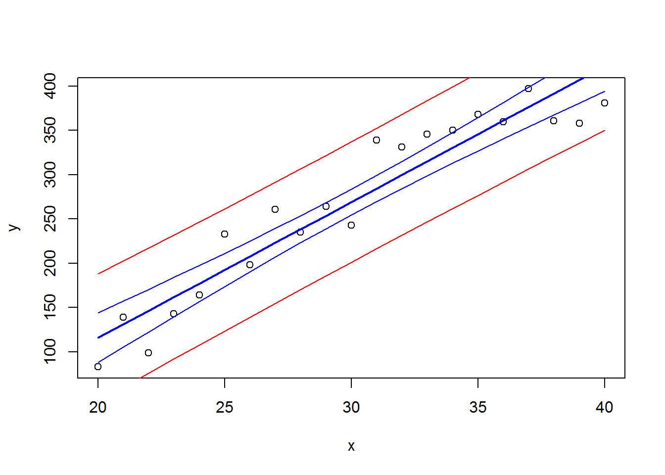
3.2.2 Multiple linear regression
Often one variable is not enough, and we need several independent variables to predict dependent one. Let’s consider internal swiss dataset: standardized fertility measure and socio-economic indicators for 47 French-speaking provinces of Switzerland at about 1888. See ?swiss
str(swiss)## 'data.frame': 47 obs. of 6 variables:
## $ Fertility : num 80.2 83.1 92.5 85.8 76.9 76.1 83.8 92.4 82.4 82.9 ...
## $ Agriculture : num 17 45.1 39.7 36.5 43.5 35.3 70.2 67.8 53.3 45.2 ...
## $ Examination : int 15 6 5 12 17 9 16 14 12 16 ...
## $ Education : int 12 9 5 7 15 7 7 8 7 13 ...
## $ Catholic : num 9.96 84.84 93.4 33.77 5.16 ...
## $ Infant.Mortality: num 22.2 22.2 20.2 20.3 20.6 26.6 23.6 24.9 21 24.4 ...## see complete model
lmAll = lm(Fertility ~ . , data = swiss)
summary(lmAll)##
## Call:
## lm(formula = Fertility ~ ., data = swiss)
##
## Residuals:
## Min 1Q Median 3Q Max
## -15.2743 -5.2617 0.5032 4.1198 15.3213
##
## Coefficients:
## Estimate Std. Error t value Pr(>|t|)
## (Intercept) 66.91518 10.70604 6.250 1.91e-07 ***
## Agriculture -0.17211 0.07030 -2.448 0.01873 *
## Examination -0.25801 0.25388 -1.016 0.31546
## Education -0.87094 0.18303 -4.758 2.43e-05 ***
## Catholic 0.10412 0.03526 2.953 0.00519 **
## Infant.Mortality 1.07705 0.38172 2.822 0.00734 **
## ---
## Signif. codes: 0 '***' 0.001 '**' 0.01 '*' 0.05 '.' 0.1 ' ' 1
##
## Residual standard error: 7.165 on 41 degrees of freedom
## Multiple R-squared: 0.7067, Adjusted R-squared: 0.671
## F-statistic: 19.76 on 5 and 41 DF, p-value: 5.594e-10## remove not significant variable
lmSig = lm(Fertility ~ . - Examination , data = swiss)
summary(lmSig)##
## Call:
## lm(formula = Fertility ~ . - Examination, data = swiss)
##
## Residuals:
## Min 1Q Median 3Q Max
## -14.6765 -6.0522 0.7514 3.1664 16.1422
##
## Coefficients:
## Estimate Std. Error t value Pr(>|t|)
## (Intercept) 62.10131 9.60489 6.466 8.49e-08 ***
## Agriculture -0.15462 0.06819 -2.267 0.02857 *
## Education -0.98026 0.14814 -6.617 5.14e-08 ***
## Catholic 0.12467 0.02889 4.315 9.50e-05 ***
## Infant.Mortality 1.07844 0.38187 2.824 0.00722 **
## ---
## Signif. codes: 0 '***' 0.001 '**' 0.01 '*' 0.05 '.' 0.1 ' ' 1
##
## Residual standard error: 7.168 on 42 degrees of freedom
## Multiple R-squared: 0.6993, Adjusted R-squared: 0.6707
## F-statistic: 24.42 on 4 and 42 DF, p-value: 1.717e-10## make simple regression using most significant variable
lm1 = lm(Fertility ~ Education , data = swiss)
summary(lm1)##
## Call:
## lm(formula = Fertility ~ Education, data = swiss)
##
## Residuals:
## Min 1Q Median 3Q Max
## -17.036 -6.711 -1.011 9.526 19.689
##
## Coefficients:
## Estimate Std. Error t value Pr(>|t|)
## (Intercept) 79.6101 2.1041 37.836 < 2e-16 ***
## Education -0.8624 0.1448 -5.954 3.66e-07 ***
## ---
## Signif. codes: 0 '***' 0.001 '**' 0.01 '*' 0.05 '.' 0.1 ' ' 1
##
## Residual standard error: 9.446 on 45 degrees of freedom
## Multiple R-squared: 0.4406, Adjusted R-squared: 0.4282
## F-statistic: 35.45 on 1 and 45 DF, p-value: 3.659e-07How to choose model? Several approaches:
- maximizing adjusted R2
- minimizing informations criteria: AIC or BIC
- Add / remove variable and compare models using likelihood ratio or chi2 test.
## calculate AIC
AIC(lm1,lmSig, lmAll)
## df AIC
## lm1 3 348.4223
## lmSig 6 325.2408
## lmAll 7 326.0716## Is fitting significnatly better? Likelihood
## simple
anova(lmAll,lmSig)## Analysis of Variance Table
##
## Model 1: Fertility ~ Agriculture + Examination + Education + Catholic +
## Infant.Mortality
## Model 2: Fertility ~ (Agriculture + Examination + Education + Catholic +
## Infant.Mortality) - Examination
## Res.Df RSS Df Sum of Sq F Pr(>F)
## 1 41 2105.0
## 2 42 2158.1 -1 -53.027 1.0328 0.3155anova(lm1,lmSig)## Analysis of Variance Table
##
## Model 1: Fertility ~ Education
## Model 2: Fertility ~ (Agriculture + Examination + Education + Catholic +
## Infant.Mortality) - Examination
## Res.Df RSS Df Sum of Sq F Pr(>F)
## 1 45 4015.2
## 2 42 2158.1 3 1857.2 12.048 7.985e-06 ***
## ---
## Signif. codes: 0 '***' 0.001 '**' 0.01 '*' 0.05 '.' 0.1 ' ' 1## more advanced
library(lmtest) ## Loading required package: zoo##
## Attaching package: 'zoo'## The following objects are masked from 'package:base':
##
## as.Date, as.Date.numericlrtest(lm1,lmSig)## Likelihood ratio test
##
## Model 1: Fertility ~ Education
## Model 2: Fertility ~ (Agriculture + Examination + Education + Catholic +
## Infant.Mortality) - Examination
## #Df LogLik Df Chisq Pr(>Chisq)
## 1 3 -171.21
## 2 6 -156.62 3 29.181 2.051e-06 ***
## ---
## Signif. codes: 0 '***' 0.001 '**' 0.01 '*' 0.05 '.' 0.1 ' ' 1lrtest(lmAll,lmSig)## Likelihood ratio test
##
## Model 1: Fertility ~ Agriculture + Examination + Education + Catholic +
## Infant.Mortality
## Model 2: Fertility ~ (Agriculture + Examination + Education + Catholic +
## Infant.Mortality) - Examination
## #Df LogLik Df Chisq Pr(>Chisq)
## 1 7 -156.04
## 2 6 -156.62 -1 1.1693 0.2796Exercises 3.2
- A biology student wishes to determine the relationship between temperature and heart rate in leopard frog, Rana pipiens. He manipulates the temperature in \(2^\circ\) increment ranging from \(2^\circ\) to \(18^\circ\)C and records the heart rate at each interval. His data are presented in table rana.txt
- Build the model and provide the p-value for linear dependency
- Provide interval estimation for the slope of the dependency
- Estimate 95% prediction interval for heart rate at 15
lm,summary,predict,confint
- Data are stored in leukemia dataset for two groups of patients who died of acute myelogenous leukemia. Patients were classified into the two groups according to the presence or absence of a morphologic characteristic of white cells. Patients termed AG positive were identified by the presence of Auer rods and/or significant granulature of the leukemic cells in the bone marrow at diagnosis. For AG-negative patients, these factors were absent. Leukemia is a cancer characterized by an overproliferation of white blood cells; the higher the white blood count (WBC), the more severe the disease. Separately for each morphologic group, AG positive and AG negative perform regression analysis of WBC-survival dependency. Consider log-transforming the data, if necessary. (Please note, that this approach is not robust… There are more advanced methods for survival analysis - see section “Survival”)
lm,summary,log
- Could you estimate
Lean.tissues.weightusing other variables of Mice dataset? Please note that there are some missing datapoints which should be excluded if you are going to compare models.
lm,summary,anova,AIC,lrtest
## 'data.frame':    790 obs. of  14 variables:
##  $ ID                  : int  1 2 3 368 369 370 371 372 4 5 ...
##  $ Strain              : Factor w/ 40 levels "129S1/SvImJ",..: 1 1 1 1 1 1 1 1 1 1 ...
##  $ Sex                 : Factor w/ 2 levels "f","m": 1 1 1 1 1 1 1 1 1 1 ...
##  $ Starting.age        : int  66 66 66 72 72 72 72 72 66 66 ...
##  $ Ending.age          : int  116 116 108 114 115 116 119 122 109 112 ...
##  $ Starting.weight     : num  19.3 19.1 17.9 18.3 20.2 18.8 19.4 18.3 17.2 19.7 ...
##  $ Ending.weight       : num  20.5 20.8 19.8 21 21.9 22.1 21.3 20.1 18.9 21.3 ...
##  $ Weight.change       : num  1.06 1.09 1.11 1.15 1.08 ...
##  $ Bleeding.time       : int  64 78 90 65 55 NA 49 73 41 129 ...
##  $ Ionized.Ca.in.blood : num  1.2 1.15 1.16 1.26 1.23 1.21 1.24 1.17 1.25 1.14 ...
##  $ Blood.pH            : num  7.24 7.27 7.26 7.22 7.3 7.28 7.24 7.19 7.29 7.22 ...
##  $ Bone.mineral.density: num  0.0605 0.0553 0.0546 0.0599 0.0623 0.0626 0.0632 0.0592 0.0513 0.0501 ...
##  $ Lean.tissues.weight : num  14.5 13.9 13.8 15.4 15.6 16.4 16.6 16 14 16.3 ...
##  $ Fat.weight          : num  4.4 4.4 2.9 4.2 4.3 4.3 5.4 4.1 3.2 5.2 ...
##
## Call:
## lm(formula = Lean.tissues.weight ~ Ending.weight, data = Mice[ikeep,
## ])
##
## Residuals:
## Min 1Q Median 3Q Max
## -12.8834 -0.9384 0.1126 1.0444 14.7162
##
## Coefficients:
## Estimate Std. Error t value Pr(>|t|)
## (Intercept) 3.09439 0.27546 11.23 <2e-16 ***
## Ending.weight 0.59811 0.01113 53.74 <2e-16 ***
## ---
## Signif. codes: 0 '***' 0.001 '**' 0.01 '*' 0.05 '.' 0.1 ' ' 1
##
## Residual standard error: 2.174 on 757 degrees of freedom
## Multiple R-squared: 0.7923, Adjusted R-squared: 0.7921
## F-statistic: 2888 on 1 and 757 DF, p-value: < 2.2e-16##
## Call:
## lm(formula = Lean.tissues.weight ~ Starting.age + Ending.age +
## Starting.weight + Ending.weight + Weight.change + Bleeding.time +
## Ionized.Ca.in.blood + Blood.pH + Bone.mineral.density + Fat.weight,
## data = Mice[ikeep, ])
##
## Residuals:
## Min 1Q Median 3Q Max
## -11.3799 -0.9078 0.1325 1.0768 13.6831
##
## Coefficients:
## Estimate Std. Error t value Pr(>|t|)
## (Intercept) 9.417619 8.757489 1.075 0.2826
## Starting.age -0.099606 0.015997 -6.226 7.95e-10 ***
## Ending.age 0.024600 0.011962 2.057 0.0401 *
## Starting.weight 0.111620 0.112864 0.989 0.3230
## Ending.weight 0.484728 0.104107 4.656 3.81e-06 ***
## Weight.change -1.478080 2.251771 -0.656 0.5118
## Bleeding.time -0.003920 0.002438 -1.608 0.1083
## Ionized.Ca.in.blood -1.324316 1.277756 -1.036 0.3003
## Blood.pH -0.386701 1.131937 -0.342 0.7327
## Bone.mineral.density 72.771474 14.096577 5.162 3.13e-07 ***
## Fat.weight 0.028885 0.033613 0.859 0.3904
## ---
## Signif. codes: 0 '***' 0.001 '**' 0.01 '*' 0.05 '.' 0.1 ' ' 1
##
## Residual standard error: 2.074 on 748 degrees of freedom
## Multiple R-squared: 0.8133, Adjusted R-squared: 0.8108
## F-statistic: 325.9 on 10 and 748 DF, p-value: < 2.2e-16##
## Call:
## lm(formula = Lean.tissues.weight ~ Starting.age + Ending.weight +
## Bone.mineral.density, data = Mice[ikeep, ])
##
## Residuals:
## Min 1Q Median 3Q Max
## -12.0505 -0.9376 0.1011 1.1112 14.5091
##
## Coefficients:
## Estimate Std. Error t value Pr(>|t|)
## (Intercept) 3.90442 0.93932 4.157 3.60e-05 ***
## Starting.age -0.06897 0.01236 -5.580 3.35e-08 ***
## Ending.weight 0.57324 0.01233 46.480 < 2e-16 ***
## Bone.mineral.density 81.49506 14.07677 5.789 1.04e-08 ***
## ---
## Signif. codes: 0 '***' 0.001 '**' 0.01 '*' 0.05 '.' 0.1 ' ' 1
##
## Residual standard error: 2.101 on 755 degrees of freedom
## Multiple R-squared: 0.8066, Adjusted R-squared: 0.8058
## F-statistic: 1049 on 3 and 755 DF, p-value: < 2.2e-16## df AIC
## res1 3 3336.880
## resSig 5 3287.060
## resAll 12 3274.053## Likelihood ratio test
##
## Model 1: Lean.tissues.weight ~ Starting.age + Ending.weight + Bone.mineral.density
## Model 2: Lean.tissues.weight ~ Starting.age + Ending.age + Starting.weight +
## Ending.weight + Weight.change + Bleeding.time + Ionized.Ca.in.blood +
## Blood.pH + Bone.mineral.density + Fat.weight
## #Df LogLik Df Chisq Pr(>Chisq)
## 1 5 -1638.5
## 2 12 -1625.0 7 27.007 0.0003323 ***
## ---
## Signif. codes: 0 '***' 0.001 '**' 0.01 '*' 0.05 '.' 0.1 ' ' 1 ![]()