- Classification, PCA and clustering
Petr V. Nazarov, LIH
2017-05-30
4.1 Classification
Let’s define 2 function:to calculate confusion matrix and stranslate it into misclassifiaction error
###############################################################
# Function that builds the confusion matrix starting from 2 vectors
# gr - target group
# gr.pred - predicted group
getConfusionMatrix = function(gr, gr.pred) {
  idx.keep = !is.na(gr) & !is.na(gr.pred)
  gr = gr[idx.keep]
  gr.pred = gr.pred[idx.keep]
    if (class(gr) == "character") gr = factor(gr); gr.pred = factor(gr.pred)
    if (class(gr) == "factor") gr = as.integer(gr); gr.pred = as.integer(gr.pred)
    n = max(c(gr, gr.pred))
    Tab = matrix(nc = n, nr = n)
    rownames(Tab) = paste("pred", 1:n, sep = ".")
    colnames(Tab) = paste("group", 1:n, sep = ".")
    for (i in 1:n){
        for (j in 1:n){
            Tab[i,j] = sum((gr.pred == i) & (gr== j))
        }
    }
    return(Tab)
}

# Function that computes the misclassification error from a confusion matrix.
getMCError = function(CM) {
    x = 0
    for (i in 1:ncol(CM))
        x = x + CM[i,i]
    return(1 - x / sum(CM))
}
4.1.1. Classification and regression
We can use logistic regression for classification: try glm with family="binomial"
Mice = read.table("http://edu.sablab.net/data/txt/mice.txt",header=T,sep="\t")
str(Mice)
## 'data.frame': 790 obs. of 14 variables:
## $ ID : int 1 2 3 368 369 370 371 372 4 5 ...
## $ Strain : Factor w/ 40 levels "129S1/SvImJ",..: 1 1 1 1 1 1 1 1 1 1 ...
## $ Sex : Factor w/ 2 levels "f","m": 1 1 1 1 1 1 1 1 1 1 ...
## $ Starting.age : int 66 66 66 72 72 72 72 72 66 66 ...
## $ Ending.age : int 116 116 108 114 115 116 119 122 109 112 ...
## $ Starting.weight : num 19.3 19.1 17.9 18.3 20.2 18.8 19.4 18.3 17.2 19.7 ...
## $ Ending.weight : num 20.5 20.8 19.8 21 21.9 22.1 21.3 20.1 18.9 21.3 ...
## $ Weight.change : num 1.06 1.09 1.11 1.15 1.08 ...
## $ Bleeding.time : int 64 78 90 65 55 NA 49 73 41 129 ...
## $ Ionized.Ca.in.blood : num 1.2 1.15 1.16 1.26 1.23 1.21 1.24 1.17 1.25 1.14 ...
## $ Blood.pH : num 7.24 7.27 7.26 7.22 7.3 7.28 7.24 7.19 7.29 7.22 ...
## $ Bone.mineral.density: num 0.0605 0.0553 0.0546 0.0599 0.0623 0.0626 0.0632 0.0592 0.0513 0.0501 ...
## $ Lean.tissues.weight : num 14.5 13.9 13.8 15.4 15.6 16.4 16.6 16 14 16.3 ...
## $ Fat.weight : num 4.4 4.4 2.9 4.2 4.3 4.3 5.4 4.1 3.2 5.2 ...## all variables except strain
mod0 = glm(Sex ~ .-Strain, data = Mice, family = "binomial")
summary(mod0)##
## Call:
## glm(formula = Sex ~ . - Strain, family = "binomial", data = Mice)
##
## Deviance Residuals:
## Min 1Q Median 3Q Max
## -2.32688 -0.67541 0.05338 0.60108 2.92236
##
## Coefficients:
## Estimate Std. Error z value Pr(>|z|)
## (Intercept) 7.714e+01 1.246e+01 6.189 6.07e-10 ***
## ID -7.552e-04 3.939e-04 -1.917 0.055213 .
## Starting.age 9.787e-03 2.302e-02 0.425 0.670684
## Ending.age 1.320e-02 1.717e-02 0.769 0.441899
## Starting.weight -4.338e-01 2.170e-01 -1.999 0.045574 *
## Ending.weight 6.482e-01 2.026e-01 3.199 0.001380 **
## Weight.change -1.106e+01 4.379e+00 -2.525 0.011554 *
## Bleeding.time -5.441e-04 3.645e-03 -0.149 0.881344
## Ionized.Ca.in.blood -1.748e+00 1.707e+00 -1.024 0.305788
## Blood.pH -7.996e+00 1.588e+00 -5.035 4.79e-07 ***
## Bone.mineral.density -3.026e+02 2.624e+01 -11.531 < 2e-16 ***
## Lean.tissues.weight 1.935e-01 5.064e-02 3.820 0.000133 ***
## Fat.weight -2.504e-02 4.502e-02 -0.556 0.578098
## ---
## Signif. codes: 0 '***' 0.001 '**' 0.01 '*' 0.05 '.' 0.1 ' ' 1
##
## (Dispersion parameter for binomial family taken to be 1)
##
## Null deviance: 1052.19 on 758 degrees of freedom
## Residual deviance: 639.57 on 746 degrees of freedom
## (31 observations deleted due to missingness)
## AIC: 665.57
##
## Number of Fisher Scoring iterations: 5## only singificant
mod1 = glm(Sex ~ Blood.pH + Bone.mineral.density + Lean.tissues.weight + Ending.weight, data = Mice, family = "binomial")
summary(mod1)##
## Call:
## glm(formula = Sex ~ Blood.pH + Bone.mineral.density + Lean.tissues.weight +
## Ending.weight, family = "binomial", data = Mice)
##
## Deviance Residuals:
## Min 1Q Median 3Q Max
## -2.32256 -0.70037 0.06679 0.65774 2.85133
##
## Coefficients:
## Estimate Std. Error z value Pr(>|z|)
## (Intercept) 51.16329 9.86196 5.188 2.13e-07 ***
## Blood.pH -6.26338 1.36317 -4.595 4.33e-06 ***
## Bone.mineral.density -267.65499 23.29329 -11.491 < 2e-16 ***
## Lean.tissues.weight 0.19641 0.04573 4.295 1.74e-05 ***
## Ending.weight 0.20287 0.03170 6.400 1.56e-10 ***
## ---
## Signif. codes: 0 '***' 0.001 '**' 0.01 '*' 0.05 '.' 0.1 ' ' 1
##
## (Dispersion parameter for binomial family taken to be 1)
##
## Null deviance: 1091.01 on 786 degrees of freedom
## Residual deviance: 704.09 on 782 degrees of freedom
## (3 observations deleted due to missingness)
## AIC: 714.09
##
## Number of Fisher Scoring iterations: 5x = predict(mod1, Mice, type="response")
x = as.factor(round(x))
CM = getConfusionMatrix(Mice$Sex,x)
print(CM)## group.1 group.2
## pred.1 307 85
## pred.2 86 309cat("Accuracy =",1 - getMCError(CM),"\n")## Accuracy = 0.78271924.1.2. Feature selections: ROC curve and AUC
Let’s consider iris dataset
library(caTools)
plot(iris[,-5],col = iris[,5],pch=19)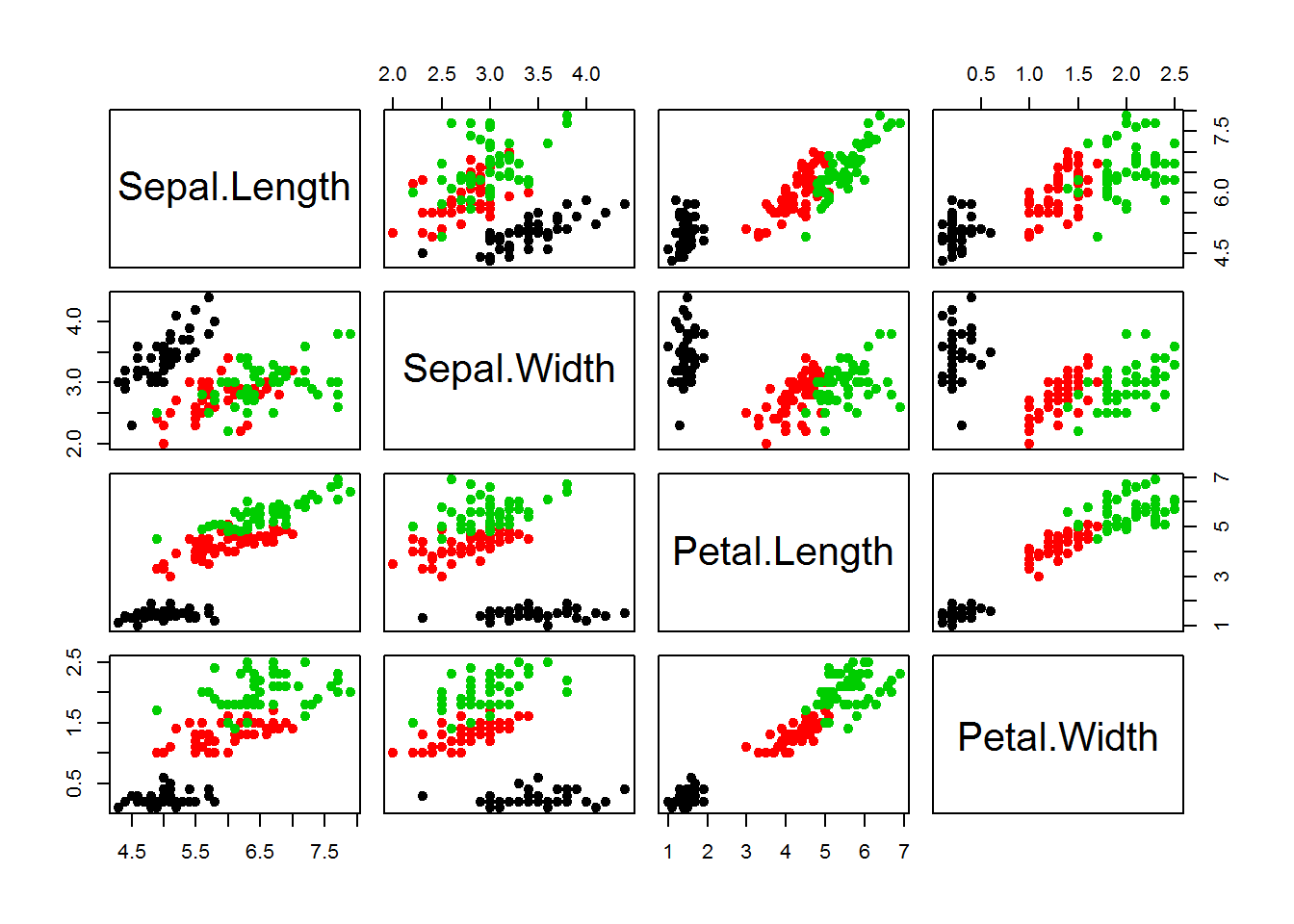
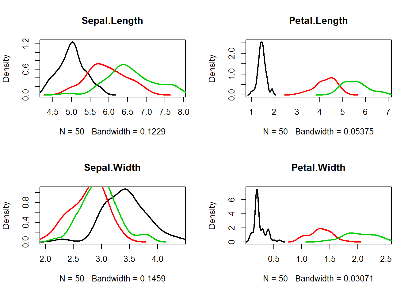
par(mfcol=c(2,2))
for (ipred in 1:4){
  plot(density(iris[as.integer(iris[,5])==1,ipred]),
       xlim=c(min(iris[,ipred]),max(iris[,ipred])),
       col=1,lwd=2,main=names(iris)[ipred])
  lines(density(iris[as.integer(iris[,5])==2,ipred]),col=2,lwd=2)
  lines(density(iris[as.integer(iris[,5])==3,ipred]),col=3,lwd=2)
}
par(mfcol=c(2,2))
colAUC(iris[,"Sepal.Length"],iris[,"Species"],plotROC=T)
## [,1]
## setosa vs. versicolor 0.9326
## setosa vs. virginica 0.9846
## versicolor vs. virginica 0.7896colAUC(iris[,"Sepal.Width"],iris[,"Species"],plotROC=T)## [,1]
## setosa vs. versicolor 0.9248
## setosa vs. virginica 0.8344
## versicolor vs. virginica 0.6636colAUC(iris[,"Petal.Length"],iris[,"Species"],plotROC=T)## [,1]
## setosa vs. versicolor 1.0000
## setosa vs. virginica 1.0000
## versicolor vs. virginica 0.9822colAUC(iris[,"Petal.Width"],iris[,"Species"],plotROC=T)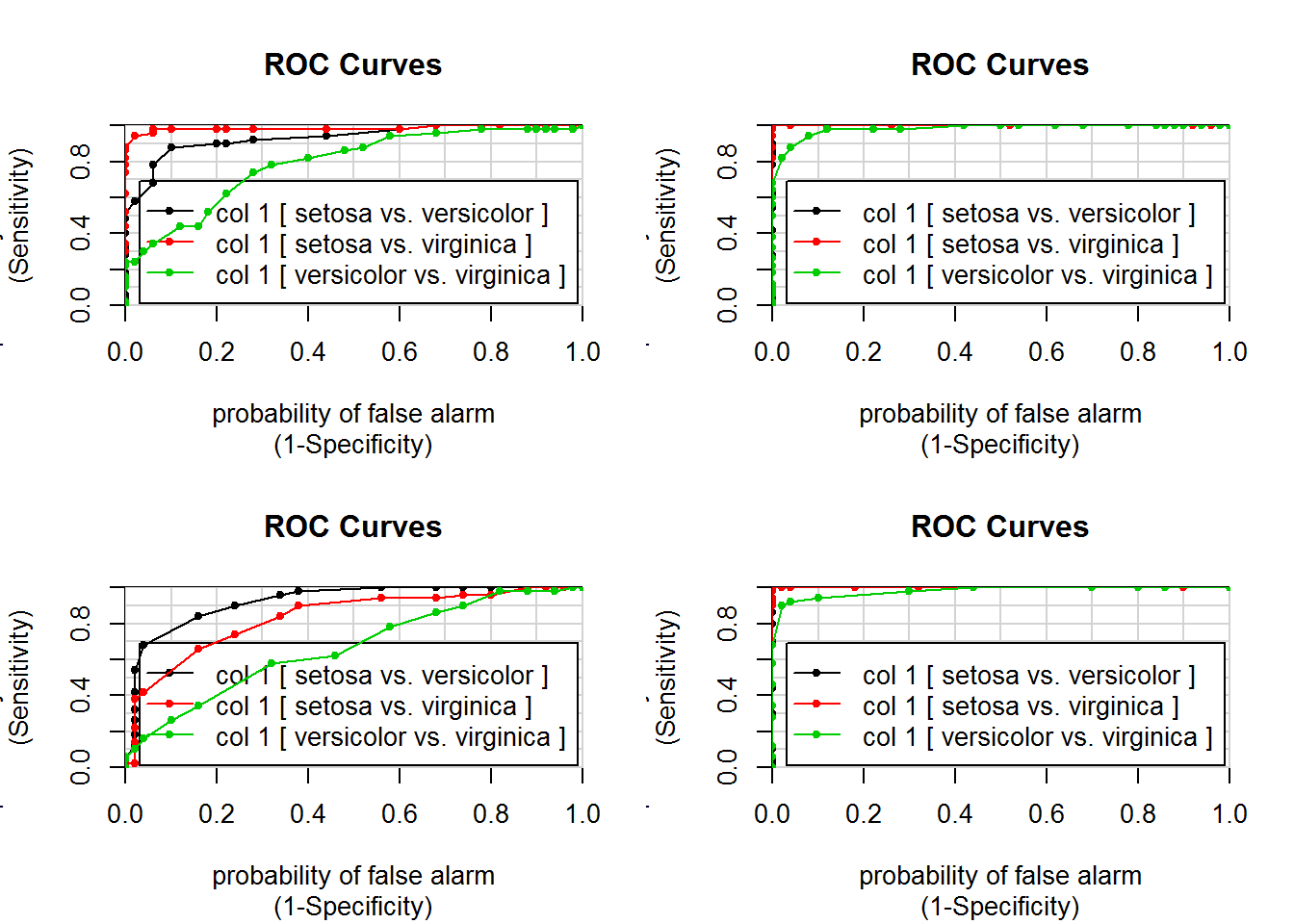
##                            [,1]
## setosa vs. versicolor    1.0000
## setosa vs. virginica     1.0000
## versicolor vs. virginica 0.9804
4.1.3. Support Vector Machine (SVM)
Let us build and validate classifier.
- We need to divide dataset into training and test subsets. For example trainging set - 70% of flowers and test set - 30%.
- Train SVM on traiing data
- Make predictions for test data and calculate misclassification error
library(e1071)##
## Attaching package: 'e1071'## The following object is masked from 'package:modeest':
##
## skewnessitrain = sample(1:nrow(iris), 0.7 * nrow(iris) )
itest = (1:nrow(iris))[-itrain]
model = svm(Species ~ ., data = iris[itrain,])
## error on training set - should be small
pred.train = as.character(predict(model,iris[itrain,-5]))
CM.train = getConfusionMatrix(iris[itrain,5], pred.train)
print(CM.train)## group.1 group.2 group.3
## pred.1 36 0 0
## pred.2 0 31 0
## pred.3 0 2 36getMCError(CM.train)## [1] 0.01904762## error on test set - much more important
pred.test = as.character(predict(model,iris[itest,-5]))
CM.test = getConfusionMatrix(iris[itest,5], pred.test)
print(CM.test)## group.1 group.2 group.3
## pred.1 14 0 0
## pred.2 0 16 2
## pred.3 0 1 12getMCError(CM.test)## [1] 0.06666667Exercises 4.1
- Please consider breast cancer dataset of Wisconsin University
breastcancer. Please note, that the data are givein in CSV format (comma-separated values). Try building glm model to discriminate benign tumours (class=0) from malignant (class=1). Play with optimal numer of predictors.
glm,getMCError,predict,getConfusionMatrix,getMCError
- For task a - train now a classifier and report correctly calculated error. Try
glmandsvm
sample,glm,svm,predict,getConfusionMatrix,getMCError
- Predict mouse gender using SVM for
micedataset and calculate the misclassification error properly
sample,svm,predict,getConfusionMatrix,getMCError
## 'data.frame':    699 obs. of  11 variables:
##  $ sample         : int  1000025 1002945 1015425 1016277 1017023 1017122 1018099 1018561 1033078 1033078 ...
##  $ clump.thickness: int  5 5 3 6 4 8 1 2 2 4 ...
##  $ uni.size       : int  1 4 1 8 1 10 1 1 1 2 ...
##  $ uni.shape      : int  1 4 1 8 1 10 1 2 1 1 ...
##  $ adhesion       : int  1 5 1 1 3 8 1 1 1 1 ...
##  $ epith.size     : int  2 7 2 3 2 7 2 2 2 2 ...
##  $ bare.nuclei    : int  1 10 2 4 1 10 10 1 1 1 ...
##  $ bland.chromatin: int  3 3 3 3 3 9 3 3 1 2 ...
##  $ normal.nucleoli: int  1 2 1 7 1 7 1 1 1 1 ...
##  $ mitoses        : int  1 1 1 1 1 1 1 1 5 1 ...
##  $ class          : int  0 0 0 0 0 1 0 0 0 0 ...
##
## Call:
## glm(formula = class ~ ., family = "binomial", data = Data)
##
## Deviance Residuals:
## Min 1Q Median 3Q Max
## -3.4877 -0.1156 -0.0613 0.0223 2.4668
##
## Coefficients:
## Estimate Std. Error z value Pr(>|z|)
## (Intercept) -1.015e+01 1.454e+00 -6.983 2.89e-12 ***
## sample 4.008e-08 7.331e-07 0.055 0.956396
## clump.thickness 5.349e-01 1.420e-01 3.767 0.000165 ***
## uni.size -6.818e-03 2.091e-01 -0.033 0.973995
## uni.shape 3.234e-01 2.307e-01 1.402 0.161010
## adhesion 3.306e-01 1.234e-01 2.679 0.007389 **
## epith.size 9.624e-02 1.567e-01 0.614 0.539233
## bare.nuclei 3.840e-01 9.546e-02 4.022 5.77e-05 ***
## bland.chromatin 4.477e-01 1.716e-01 2.608 0.009099 **
## normal.nucleoli 2.134e-01 1.131e-01 1.887 0.059224 .
## mitoses 5.344e-01 3.294e-01 1.622 0.104740
## ---
## Signif. codes: 0 '***' 0.001 '**' 0.01 '*' 0.05 '.' 0.1 ' ' 1
##
## (Dispersion parameter for binomial family taken to be 1)
##
## Null deviance: 884.35 on 682 degrees of freedom
## Residual deviance: 102.89 on 672 degrees of freedom
## (16 observations deleted due to missingness)
## AIC: 124.89
##
## Number of Fisher Scoring iterations: 8## group.1 group.2
## pred.1 434 11
## pred.2 10 228## Accuracy = 0.96925334.2. PCA
## clear memory
rm(list = ls())

## Let's transform iris data frame into numerical matrix
## data - numerical data
## classes - type of iris, 1=setosa, 2=versicolor, 3=virginica
Data = as.matrix(iris[,-5])
row.names(Data) = as.character(iris[,5])
classes = as.integer(iris[,5])

## perform PCA. We need data to be a matrix
PC = prcomp(Data)
str(PC)
## List of 5
## $ sdev : num [1:4] 2.056 0.493 0.28 0.154
## $ rotation: num [1:4, 1:4] 0.3614 -0.0845 0.8567 0.3583 -0.6566 ...
## ..- attr(*, "dimnames")=List of 2
## .. ..$ : chr [1:4] "Sepal.Length" "Sepal.Width" "Petal.Length" "Petal.Width"
## .. ..$ : chr [1:4] "PC1" "PC2" "PC3" "PC4"
## $ center : Named num [1:4] 5.84 3.06 3.76 1.2
## ..- attr(*, "names")= chr [1:4] "Sepal.Length" "Sepal.Width" "Petal.Length" "Petal.Width"
## $ scale : logi FALSE
## $ x : num [1:150, 1:4] -2.68 -2.71 -2.89 -2.75 -2.73 ...
## ..- attr(*, "dimnames")=List of 2
## .. ..$ : chr [1:150] "setosa" "setosa" "setosa" "setosa" ...
## .. ..$ : chr [1:4] "PC1" "PC2" "PC3" "PC4"
## - attr(*, "class")= chr "prcomp"## plot PC1 and PC2 only
plot(PC$x[,1],PC$x[,2],col=classes, pch=19)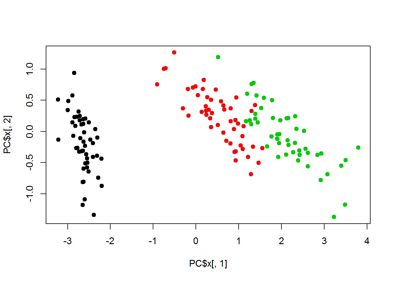
## plot in 3D
library(rgl)
plot3d(PC$x[,1],PC$x[,2],PC$x[,3],
       size = 2,
       col  = classes,
       type = "s",
       xlab = "PC1",
       ylab = "PC2",
       zlab = "PC3")

##--------------------------------------
## PCA for Mice

Mice = read.table("http://edu.sablab.net/data/txt/mice.txt", header=T,sep="\t")
Mice = na.omit(Mice)
Data=as.matrix(Mice[,-(1:5)])
PC = prcomp(Data,scale=TRUE)
## TRUE - will capture technical outliers (absent values)
## FALSE - will capture mailny bleding time

str(PC)
## List of 5
## $ sdev : num [1:9] 1.984 1.084 1.014 0.967 0.912 ...
## $ rotation: num [1:9, 1:9] 0.467 0.488 0.135 -0.105 0.148 ...
## ..- attr(*, "dimnames")=List of 2
## .. ..$ : chr [1:9] "Starting.weight" "Ending.weight" "Weight.change" "Bleeding.time" ...
## .. ..$ : chr [1:9] "PC1" "PC2" "PC3" "PC4" ...
## $ center : Named num [1:9] 21.42 23.71 1.11 61.02 1.24 ...
## ..- attr(*, "names")= chr [1:9] "Starting.weight" "Ending.weight" "Weight.change" "Bleeding.time" ...
## $ scale : Named num [1:9] 6.001 7.096 0.106 31.936 0.062 ...
## ..- attr(*, "names")= chr [1:9] "Starting.weight" "Ending.weight" "Weight.change" "Bleeding.time" ...
## $ x : num [1:759, 1:9] -0.6027 -1.0013 -1.3816 -0.3864 -0.0464 ...
## ..- attr(*, "dimnames")=List of 2
## .. ..$ : chr [1:759] "1" "2" "3" "4" ...
## .. ..$ : chr [1:9] "PC1" "PC2" "PC3" "PC4" ...
## - attr(*, "class")= chr "prcomp"## plot PC1 and PC2 only
col=c("#AA002255","#0000AA55")
plot(PC$x[,1],PC$x[,2],col=col[Mice$Sex], pch=19)
text(PC$x[,1],PC$x[,2]-0.5,Mice$ID,cex=0.6,col="#000000AA")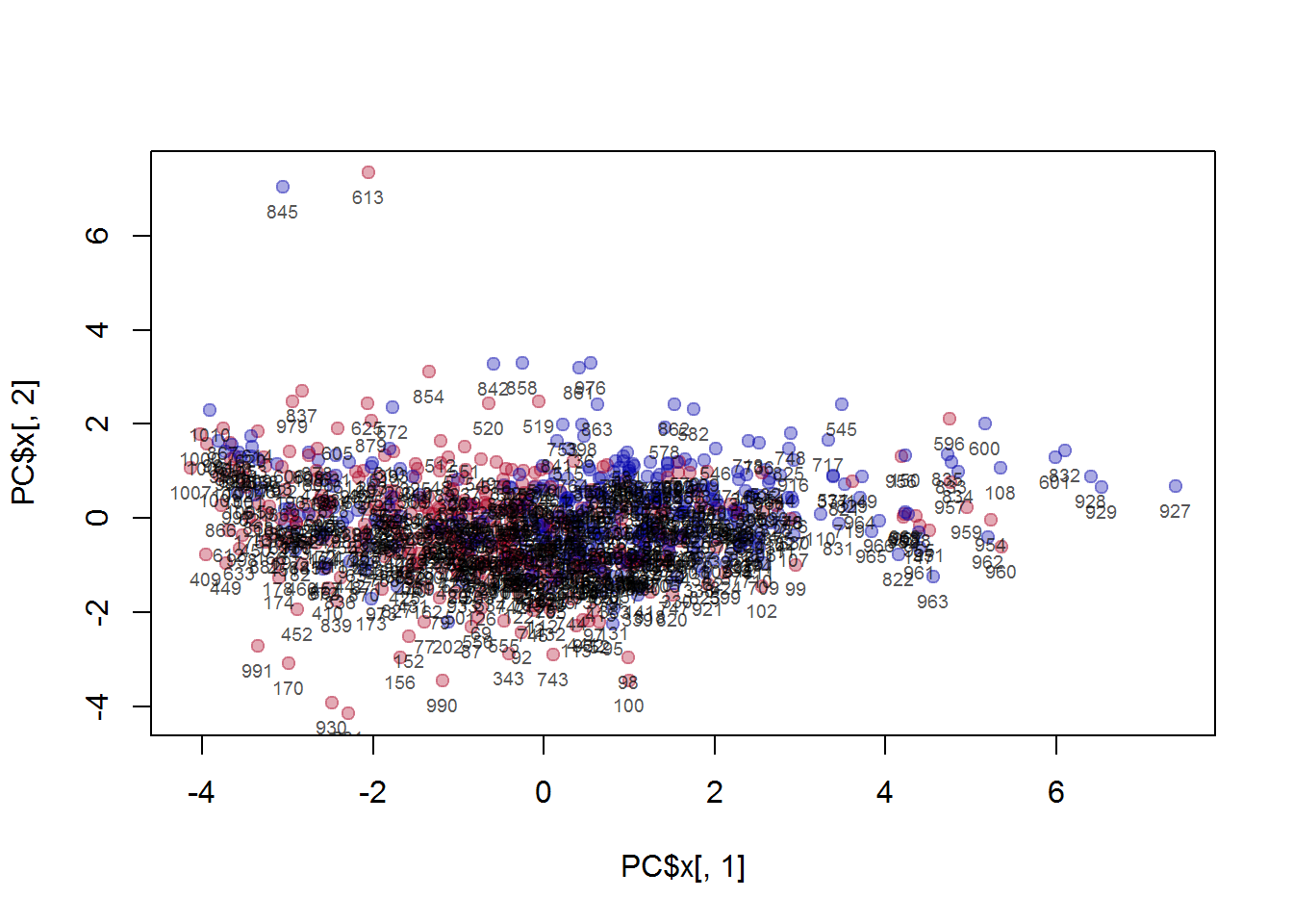
## investigate manually the outliers
Mice[Mice$ID %in% c(845,613),]
## ID Strain Sex Starting.age Ending.age Starting.weight
## 318 613 CZECHII/EiJ f 69 113 10.1
## 412 845 JF1/Ms m 53 107 16.4
## Ending.weight Weight.change Bleeding.time Ionized.Ca.in.blood Blood.pH
## 318 21.3 2.109 57 1.17 7.05
## 412 20.3 1.238 522 1.13 7.43
## Bone.mineral.density Lean.tissues.weight Fat.weight
## 318 0.0419 8.0 1.8
## 412 0.0461 11.7 4.1##----------------------------------------
## PCA for ALL
ALL = read.table("http://edu.sablab.net/data/txt/all_data.txt", as.is=T,header=T,sep="\t")
str(ALL) ## see here - experiments are in columns!!!## 'data.frame': 15391 obs. of 57 variables:
## $ ID : chr "A1BG" "A1CF" "A2BP1" "A2LD1" ...
## $ Name : chr "alpha-1-B glycoprotein" "APOBEC1 complementation factor" "ataxin 2-binding protein 1" "AIG2-like domain 1" ...
## $ ALL_GSM51674 : num 5.17 6.16 6.89 5.82 6.1 ...
## $ ALL_GSM51675 : num 5.36 6.01 6.42 5.81 6.14 ...
## $ ALL_GSM51676 : num 5.42 5.75 6.74 5.52 6.16 ...
## $ ALL_GSM51677 : num 5.23 6.12 6.07 5.6 6.1 ...
## $ ALL_GSM51678 : num 5.63 6.57 6.58 5.66 6.34 ...
## $ ALL_GSM51679 : num 5.3 5.68 6.44 5.84 5.88 ...
## $ ALL_GSM51680 : num 5.72 5.95 6.52 5.81 6.05 ...
## $ ALL_GSM51681 : num 5.33 5.93 6.58 5.88 5.71 ...
## $ ALL_GSM51682 : num 5.37 5.78 5.9 5.7 5.91 ...
## $ ALL_GSM51683 : num 5.8 5.13 6.16 5.69 5.6 ...
## $ ALL_GSM51684 : num 5.58 5.84 6.36 5.55 6.19 ...
## $ ALL_GSM51685 : num 6.32 7.13 7.08 6.18 6.65 ...
## $ ALL_GSM51686 : num 5.85 6.9 7.59 6.58 6.91 ...
## $ ALL_GSM51687 : num 5.93 7.15 7.44 6.41 6.74 ...
## $ ALL_GSM51688 : num 5.34 7.98 8.02 6.89 7.13 ...
## $ ALL_GSM51689 : num 5.74 8 7.89 6.82 6.71 ...
## $ ALL_GSM51690 : num 6.92 5.3 6.9 5.52 5.9 ...
## $ ALL_GSM51691 : num 6.12 5.26 5.84 5.42 5.64 ...
## $ ALL_GSM51692 : num 6.99 5.82 6.13 5.69 5.32 ...
## $ ALL_GSM51693 : num 6.06 5.28 5.93 5.52 5.68 ...
## $ ALL_GSM51694 : num 6.16 5.62 6.27 4.89 5.83 ...
## $ ALL_GSM51695 : num 6.1 5.33 5.75 5.38 5.8 ...
## $ ALL_GSM51696 : num 6.31 4.98 6.1 4.71 5.93 ...
## $ ALL_GSM51697 : num 6.07 5.28 5.93 5.21 5.93 ...
## $ ALL_GSM51698 : num 6.21 5.02 5.81 5.05 5.8 ...
## $ ALL_GSM51699 : num 6.87 5.63 6.36 5.39 5.71 ...
## $ ALL_GSM51700 : num 6.62 5.43 5.87 4.79 5.58 ...
## $ ALL_GSM51701 : num 6.78 5.68 6.2 5.27 5.69 ...
## $ ALL_GSM51702 : num 7.01 4.91 6.08 5.41 7.02 ...
## $ ALL_GSM51703 : num 6.19 5.17 5.83 5.42 6.41 ...
## $ ALL_GSM51704 : num 6.29 5.26 5.83 5.19 6.68 ...
## $ ALL_GSM51705 : num 6.75 5.27 5.63 5.37 6.6 ...
## $ ALL_GSM51706 : num 6.38 5.22 5.78 5.36 6.43 ...
## $ ALL_GSM51707 : num 6.46 5.84 6.51 5.35 6.26 ...
## $ ALL_GSM51708 : num 6.17 5.12 6.15 5.49 5.72 ...
## $ ALL_GSM51709 : num 6.29 5.46 6.05 5.58 5.67 ...
## $ ALL_GSM51710 : num 6.98 5.02 6.07 5.91 5.85 ...
## $ ALL_GSM51711 : num 6.45 4.89 5.79 5.79 5.77 ...
## $ ALL_GSM51712 : num 6.56 5.31 5.9 5.49 5.76 ...
## $ normal_GSM270834: num 6.22 5.26 6.09 5.58 5.8 ...
## $ normal_GSM270835: num 6.5 5.01 5.98 5.46 5.75 ...
## $ normal_GSM270836: num 6.21 4.96 6.19 5.39 5.74 ...
## $ normal_GSM270837: num 6.45 5.19 6.15 5.64 5.71 ...
## $ normal_GSM270838: num 5.67 5.5 6.44 5.61 6.54 ...
## $ normal_GSM270839: num 6.58 5.7 5.95 5.2 6.02 ...
## $ normal_GSM270840: num 6.98 5.09 6.07 5.23 5.85 ...
## $ normal_GSM270841: num 6.92 5.48 5.71 5.43 5.66 ...
## $ normal_GSM270842: num 6.77 4.98 5.95 5.44 5.71 ...
## $ normal_GSM270843: num 6.74 5.34 6.22 5.6 5.63 ...
## $ normal_GSM270844: num 7.32 5.62 6.18 5.26 5.68 ...
## $ normal_GSM50698 : num 7.05 5.38 6.06 5.27 5.67 ...
## $ normal_GSM50699 : num 6.91 5.65 5.93 5.05 5.87 ...
## $ normal_GSM50700 : num 6.54 4.86 6.15 5.67 5.71 ...
## $ normal_GSM50701 : num 6.28 5.9 5.87 5.72 5.36 ...
## $ normal_GSM50702 : num 6.62 5.39 6.28 5.85 5.72 ...## Transform to matrix
Data=as.matrix(ALL[,-(1:2)])
## assign colors based on column names
color = colnames(Data)
color[grep("ALL",color)]="red"
color[grep("normal",color)]="blue"
## perform PCA
PC = prcomp(t(Data))
## visualize in 3D
library(rgl)
plot3d(PC$x[,1],PC$x[,2],PC$x[,3],size = 2,col = color,type = "s",
xlab = "PC1",ylab = "PC2",zlab = "PC3")
## plot PC1 and PC2 only
plot(PC$x[,1],PC$x[,2],col=color,pch=19,cex=2)
text(PC$x[,1],PC$x[,2]+5,colnames(Data),cex=0.6)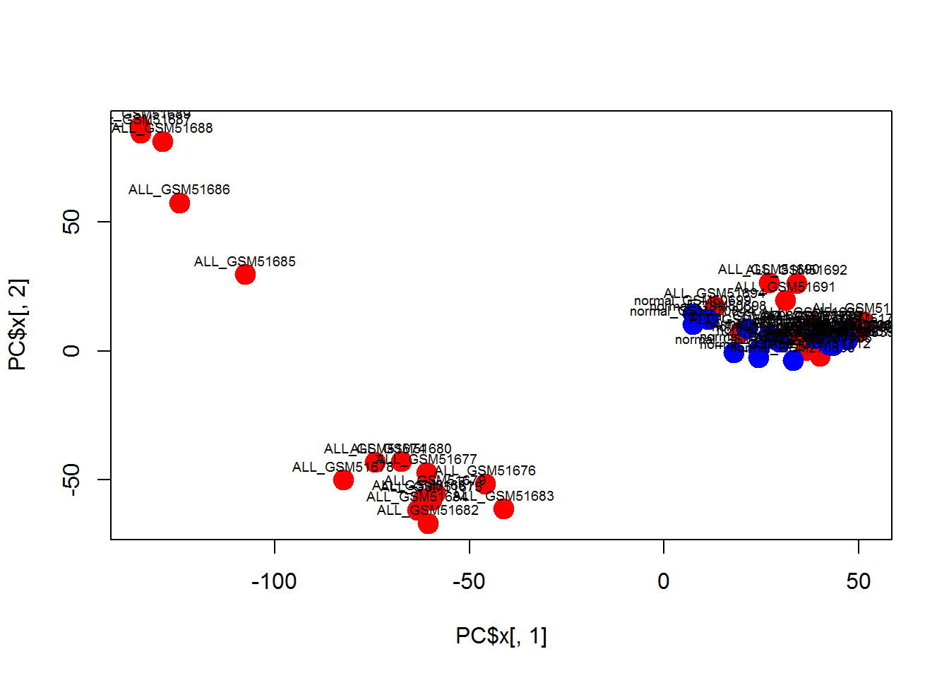
PCG = prcomp(Data)
plot(PCG$x[,1],PCG$x[,2],col="#00FF0011",pch=19,cex=2)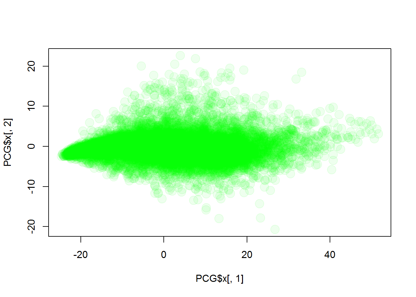
plot3d(PCG$x[,1],PCG$x[,2],PCG$x[,3],size = 1,col  = "green",type = "s",
       xlab = "PC1",ylab = "PC2",zlab = "PC3")

## check the distribution of the data
source("http://sablab.net/scripts/plotDataPDF.r")
plotDataPDF(Data,col=color,add.legend=T)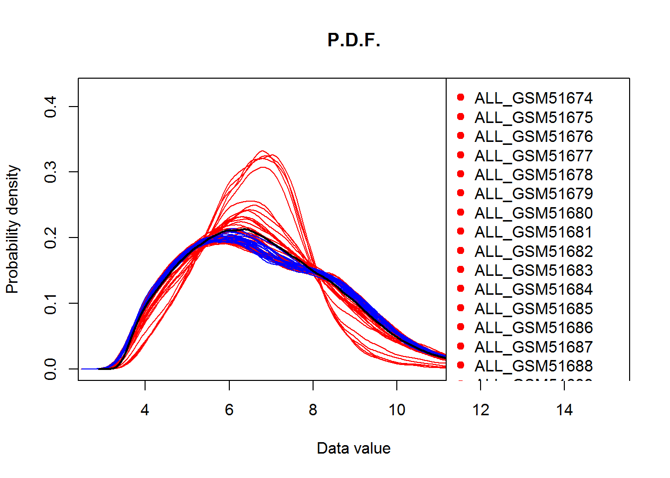
boxplot(Data,col=color,outline=F,las=2)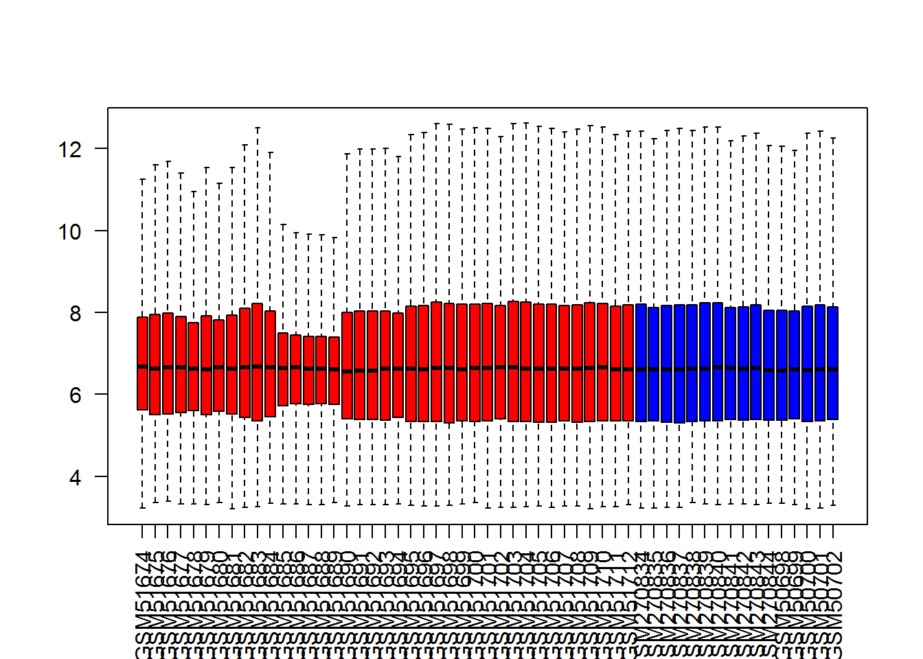
Exercises 4.2
- Work with mice data from http://edu.sablab.net/data/txt/mice.txt. Perform PCA and identify outliers (or strangely behaving creatures) among mice population. Hint: Replace NA values in each column by the corresponding median value (for this column).
prcomp
- Acute lymphoblastic leukemia (ALL), is a form of leukemia characterized by excess lymphoblasts. ALL contains the results of transcriptome profiling for ALL patients and healthy donors using Affymetrix microarrays. The expression values in the table are in log2 scale. See data at http://edu.sablab.net/data/txt/all_data.txt
Perform exploratory analysis of ALL dataset using PCA
4.3. Clustering
##------------------------------------
## k-means Clustering
Data = as.matrix(iris[,-5])
row.names(Data) = as.character(iris[,5])
classes = as.integer(iris[,5])

## try k-means clustering
clusters = kmeans(x=Data,centers=3,nstart=10)$cluster

## show clusters on PCA
PC = prcomp(Data)
plot(PC$x[,1],PC$x[,2],col = classes,pch=clusters)
legend(2,1.4,levels(iris$Species),col=c(1,2,3),pch=19)
legend(-2.5,1.4,c("c1","c2","c3"),col=4,pch=c(1,2,3))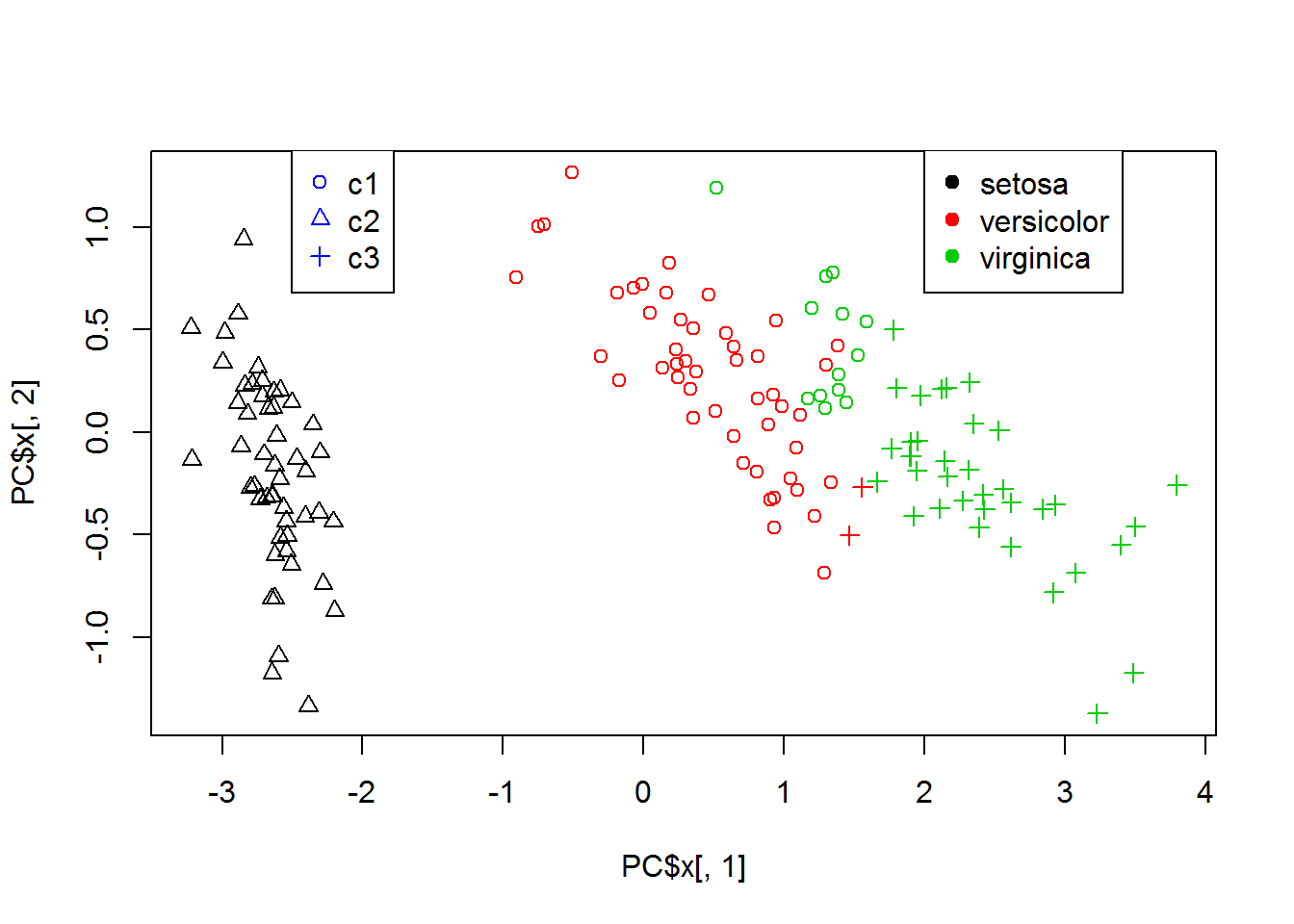
##-----------------------------------------
## Hierarchical clustering

## use heatmap
heatmap(Data)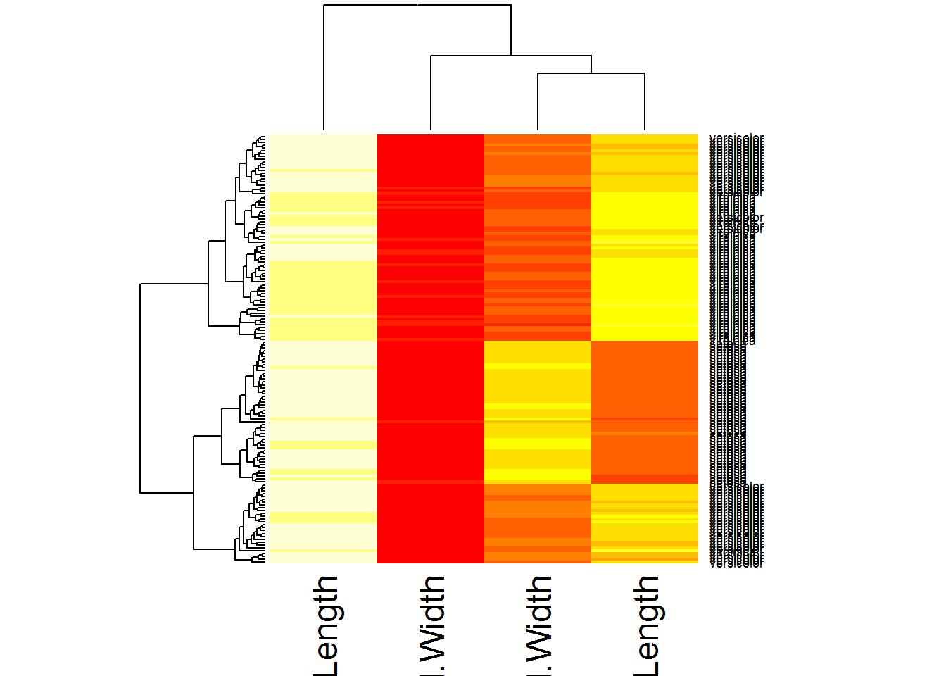
## use heatmap with colors
color = character(length(classes))
color[classes == 1] = "black"
color[classes == 2] = "red"
color[classes == 3] = "green"
heatmap(Data,RowSideColors=color,scale="none")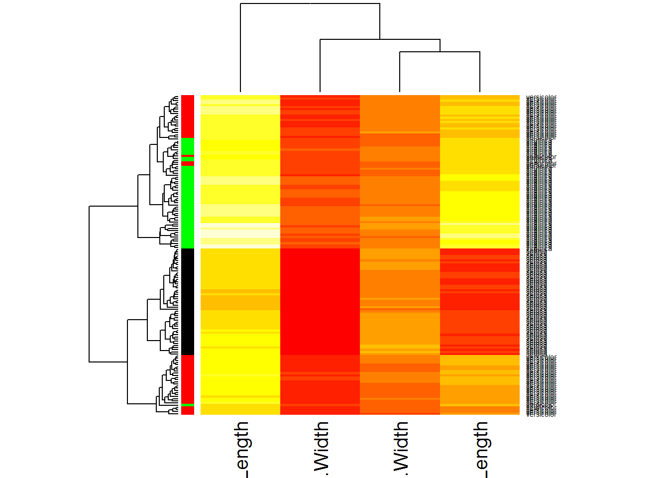
## modify the heatmap colors
heatmap(Data,RowSideColors=color,scale="none",col = colorRampPalette (c("blue","wheat","red"))(1000))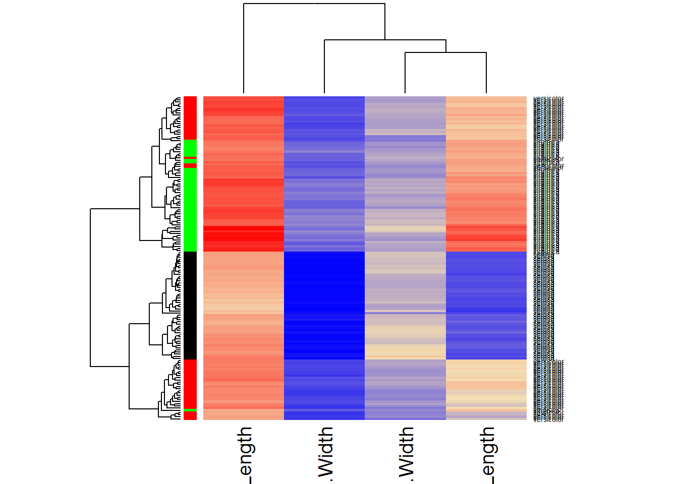
## Another heatmap:
library(gplots)
##
## Attaching package: 'gplots'## The following object is masked from 'package:stats':
##
## lowessheatmap.2(Data,RowSideColors=color,scale="none",trace="none",
col = colorRampPalette (c("blue","wheat","red"))(1000))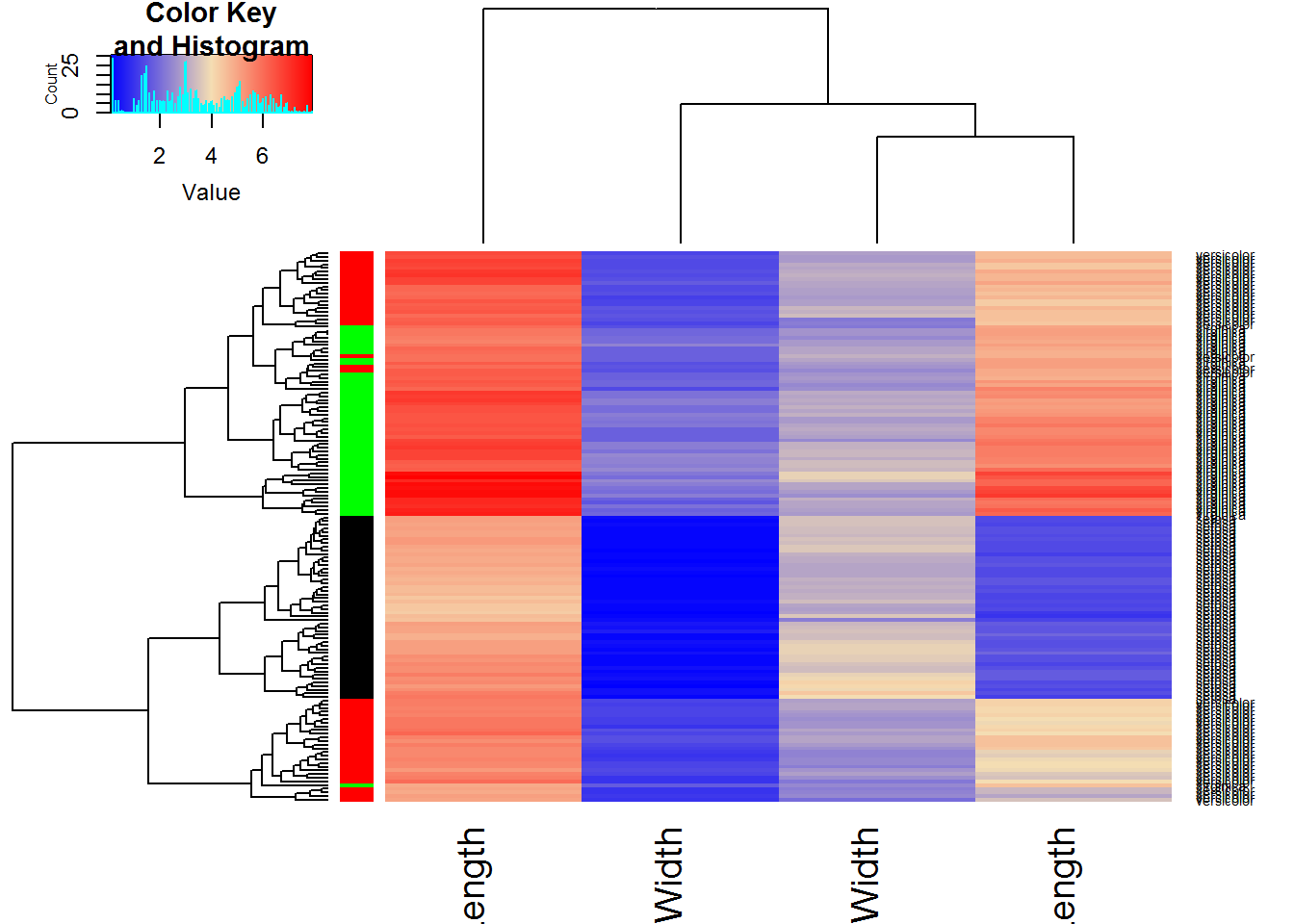
plot(hclust(dist(Data)))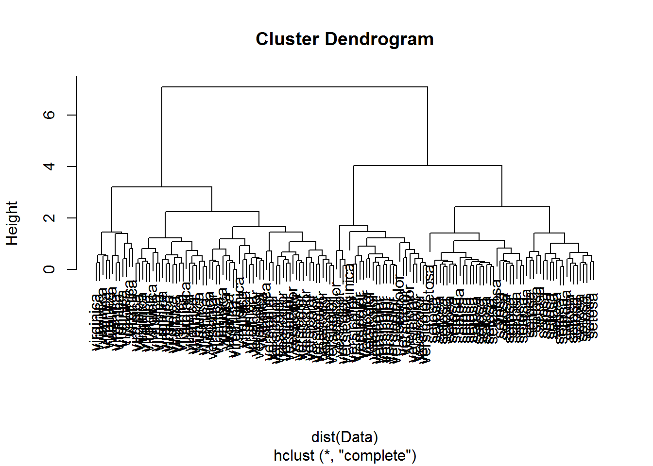
##------------------------------------------------------------------------------
## Hierarchical clustering: ALL
##------------------------------------------------------------------------------
ALL = read.table("http://edu.sablab.net/data/txt/all_data.txt",
                  as.is=T,header=T,sep="\t")
Data=as.matrix(ALL[,-(1:2)])
color = colnames(Data)
color[grep("ALL",color)]="red"
color[grep("normal",color)]="blue"
##----------------------------------
## Task L5.2a. Select top 100 genes

## annotate genes
rownames(Data) = ALL[,1]
## create indexes for normal and ALL columns
idx.norm = grep("normal",colnames(Data))
idx.all = grep("ALL",colnames(Data))

## perform a t-test
pv = double(nrow(Data))
for (i in 1:nrow(Data)){
  pv[i] = t.test(Data[i,idx.all],Data[i,idx.norm])$p.val
}
## select top genes
Top = Data[order(pv),][1:100,]

## make a heatmap
heatmap(Top,ColSideColors=color,
          col = colorRampPalette (c("blue","wheat","red"))(1000))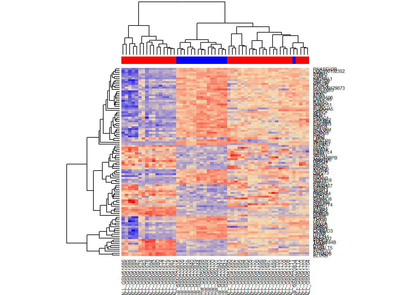
## scale data first and repeat heatmap
TopSc = t(scale(t(Top)))
heatmap(TopSc,ColSideColors=color,
          col = colorRampPalette (c("blue","white","red"))(1000))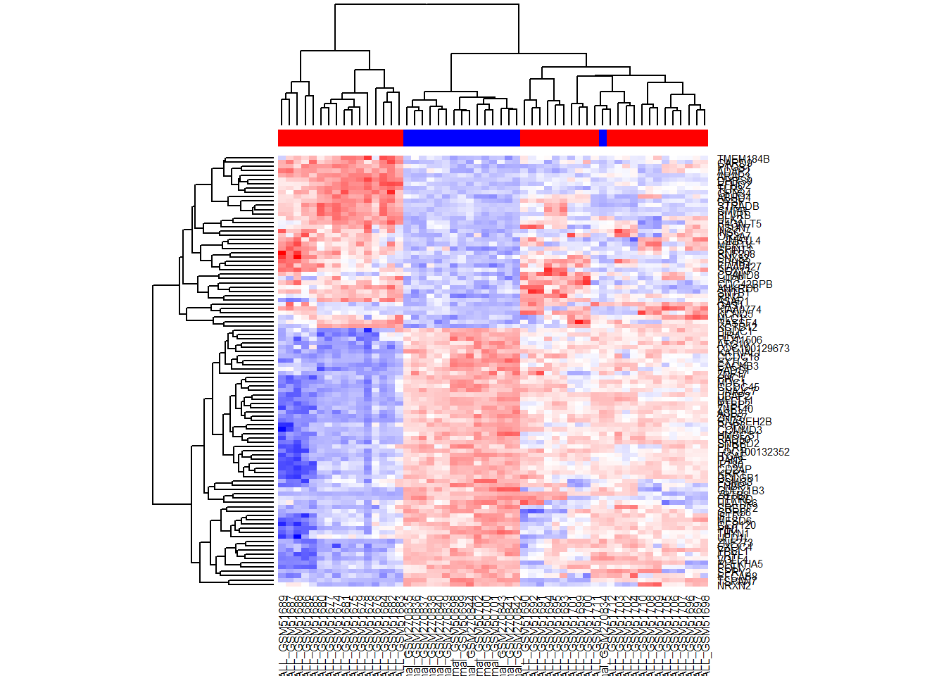
library(gplots)
heatmap.2(TopSc,ColSideColors=color,trace="none",
          col = colorRampPalette (c("blue","white","red"))(1000))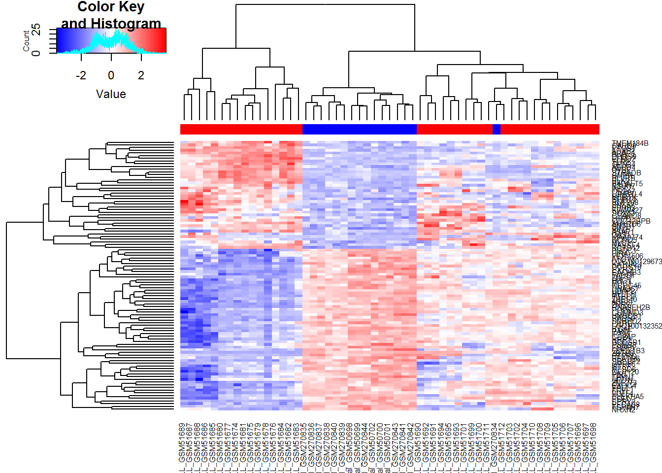
library(pheatmap)
pheatmap(TopSc)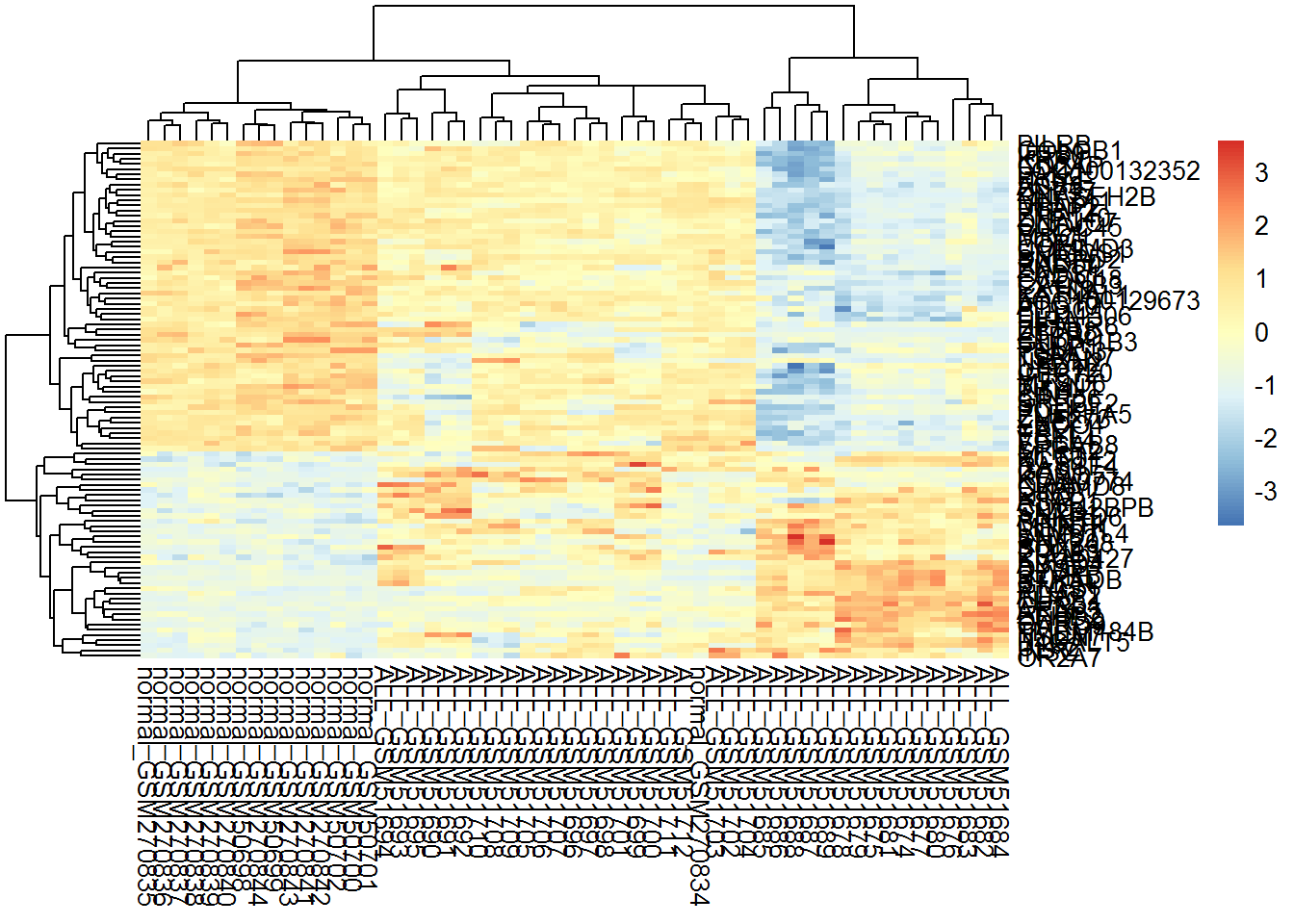
Exercises 4.2-4.3
Work with qPCR Taqman dataset. This dataset contains CT values for microRNAs detected in several samples under two conditions. Note, that higher CT is, lower is the RNA abundance. Please, load and clean the data. Replace NA by the maximum detected CT value Build kmeans and hierarchical clustering for these genes, visualize by PCA
![]()