- Multiple comparisons. Survival Analysis
Petr V. Nazarov, LIH
2017-05-31
5.1. Multiple Comparisons
rm(list=ls())
## define data size
nsamples = 6
nfeatures = 1000 ## "genes"

## create random data
D = matrix(rnorm(nsamples*nfeatures), nrow=nfeatures, ncol=nsamples)
## vector of p-values
pv = double(nfeatures)

## let's apply t.test to each feature (gene)
## comparing 1,2,3 columns to 4,5,6
for (i in 1:nfeatures){
  pv[i] = t.test(D[i,1:3],D[i,4:6])$p.value
}
## count number of 'significant' p-values
sum(pv < 0.05)
## [1] 31par(mfcol=c(2,4))
for (i in which(pv < 0.01)){
plot(D[i,],col=c(2,2,2,4,4,4),pch=19,cex=2)
}
## make FDR adjustment...
par(mfcol=c(1,1))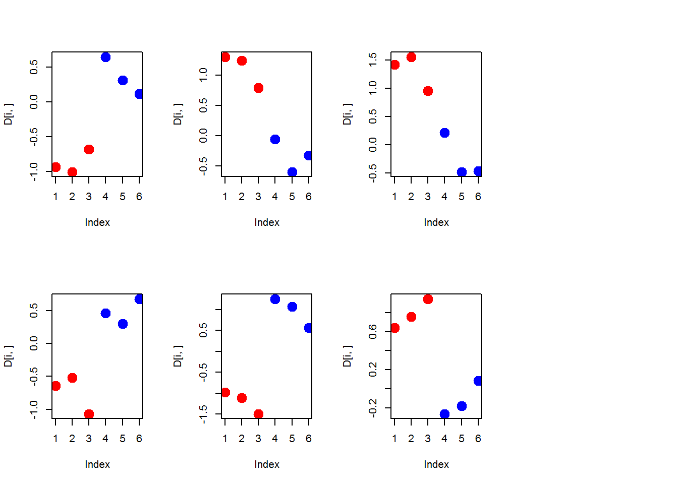
sum(p.adjust(pv, method="fdr")<0.05)## [1] 0plot(pv, p.adjust(pv, method="fdr"))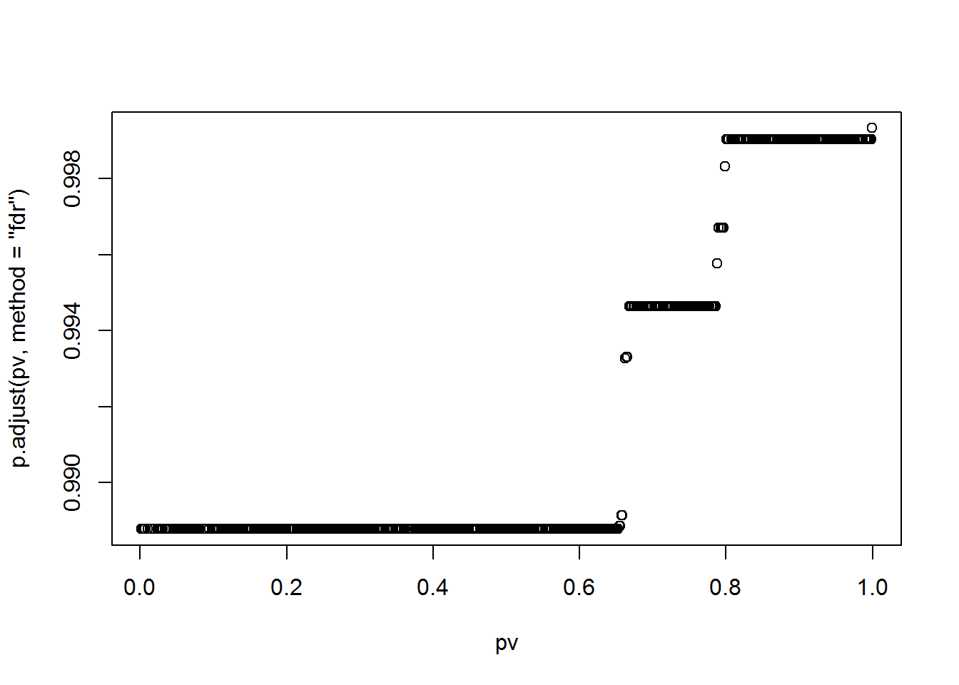
5.2. Survival Analysis
rm(list=ls())
library(survival)
str(lung)
## 'data.frame': 228 obs. of 10 variables:
## $ inst : num 3 3 3 5 1 12 7 11 1 7 ...
## $ time : num 306 455 1010 210 883 ...
## $ status : num 2 2 1 2 2 1 2 2 2 2 ...
## $ age : num 74 68 56 57 60 74 68 71 53 61 ...
## $ sex : num 1 1 1 1 1 1 2 2 1 1 ...
## $ ph.ecog : num 1 0 0 1 0 1 2 2 1 2 ...
## $ ph.karno : num 90 90 90 90 100 50 70 60 70 70 ...
## $ pat.karno: num 100 90 90 60 90 80 60 80 80 70 ...
## $ meal.cal : num 1175 1225 NA 1150 NA ...
## $ wt.loss : num NA 15 15 11 0 0 10 1 16 34 ...## create a survival object
## lung$status: 1-censored, 2-dead
sData = Surv(lung$time,event = lung$status == 2)
print(sData)## [1] 306 455 1010+ 210 883 1022+ 310 361 218 166 170
## [12] 654 728 71 567 144 613 707 61 88 301 81
## [23] 624 371 394 520 574 118 390 12 473 26 533
## [34] 107 53 122 814 965+ 93 731 460 153 433 145
## [45] 583 95 303 519 643 765 735 189 53 246 689
## [56] 65 5 132 687 345 444 223 175 60 163 65
## [67] 208 821+ 428 230 840+ 305 11 132 226 426 705
## [78] 363 11 176 791 95 196+ 167 806+ 284 641 147
## [89] 740+ 163 655 239 88 245 588+ 30 179 310 477
## [100] 166 559+ 450 364 107 177 156 529+ 11 429 351
## [111] 15 181 283 201 524 13 212 524 288 363 442
## [122] 199 550 54 558 207 92 60 551+ 543+ 293 202
## [133] 353 511+ 267 511+ 371 387 457 337 201 404+ 222
## [144] 62 458+ 356+ 353 163 31 340 229 444+ 315+ 182
## [155] 156 329 364+ 291 179 376+ 384+ 268 292+ 142 413+
## [166] 266+ 194 320 181 285 301+ 348 197 382+ 303+ 296+
## [177] 180 186 145 269+ 300+ 284+ 350 272+ 292+ 332+ 285
## [188] 259+ 110 286 270 81 131 225+ 269 225+ 243+ 279+
## [199] 276+ 135 79 59 240+ 202+ 235+ 105 224+ 239 237+
## [210] 173+ 252+ 221+ 185+ 92+ 13 222+ 192+ 183 211+ 175+
## [221] 197+ 203+ 116 188+ 191+ 105+ 174+ 177+## Let's visualize it
fit = survfit(sData~1)
plot(fit)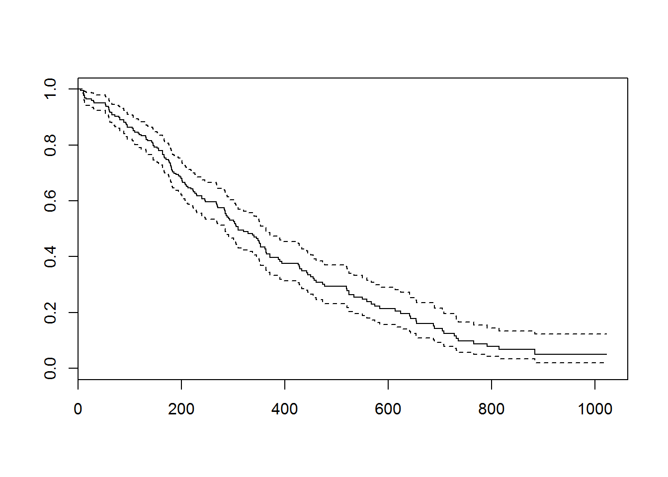
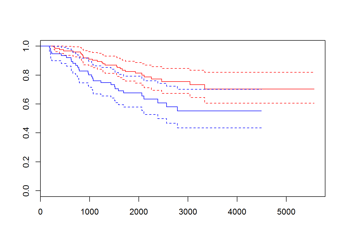
## Let's visualize it for male/female
fit.sex = survfit(sData ~ lung$sex)
plot(fit.sex, col=c("blue","red"), conf.int = TRUE, mark.time=TRUE)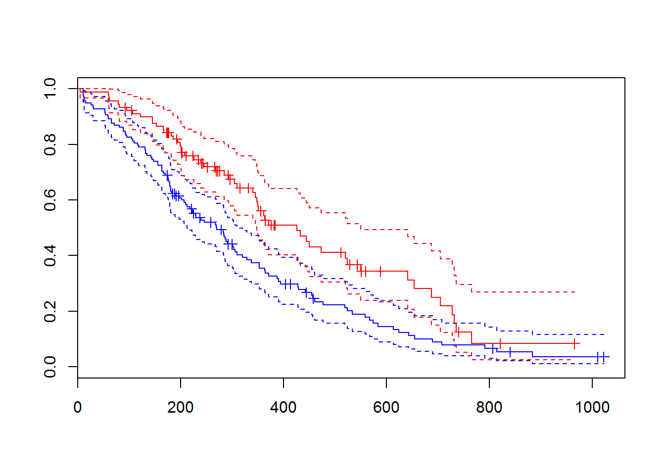
str(fit.sex)## List of 14
## $ n : int [1:2] 138 90
## $ time : num [1:206] 11 12 13 15 26 30 31 53 54 59 ...
## $ n.risk : num [1:206] 138 135 134 132 131 130 129 128 126 125 ...
## $ n.event : num [1:206] 3 1 2 1 1 1 1 2 1 1 ...
## $ n.censor : num [1:206] 0 0 0 0 0 0 0 0 0 0 ...
## $ surv : num [1:206] 0.978 0.971 0.957 0.949 0.942 ...
## $ type : chr "right"
## $ strata : Named int [1:2] 119 87
## ..- attr(*, "names")= chr [1:2] "lung$sex=1" "lung$sex=2"
## $ std.err : num [1:206] 0.0127 0.0147 0.0181 0.0197 0.0211 ...
## $ upper : num [1:206] 1 0.999 0.991 0.987 0.982 ...
## $ lower : num [1:206] 0.954 0.943 0.923 0.913 0.904 ...
## $ conf.type: chr "log"
## $ conf.int : num 0.95
## $ call : language survfit(formula = sData ~ lung$sex)
## - attr(*, "class")= chr "survfit"## Rank test for survival data
dif.sex = survdiff(sData ~ lung$sex)
dif.sex## Call:
## survdiff(formula = sData ~ lung$sex)
##
## N Observed Expected (O-E)^2/E (O-E)^2/V
## lung$sex=1 138 112 91.6 4.55 10.3
## lung$sex=2 90 53 73.4 5.68 10.3
##
## Chisq= 10.3 on 1 degrees of freedom, p= 0.00131str(dif.sex)## List of 6
## $ n : 'table' int [1:2(1d)] 138 90
## ..- attr(*, "dimnames")=List of 1
## .. ..$ groups: chr [1:2] "lung$sex=1" "lung$sex=2"
## $ obs : num [1:2] 112 53
## $ exp : num [1:2] 91.6 73.4
## $ var : num [1:2, 1:2] 40.4 -40.4 -40.4 40.4
## $ chisq: num 10.3
## $ call : language survdiff(formula = sData ~ lung$sex)
## - attr(*, "class")= chr "survdiff"## build Cox regression model
mod1 = coxph(sData ~ sex, data=lung)
summary(mod1)## Call:
## coxph(formula = sData ~ sex, data = lung)
##
## n= 228, number of events= 165
##
## coef exp(coef) se(coef) z Pr(>|z|)
## sex -0.5310 0.5880 0.1672 -3.176 0.00149 **
## ---
## Signif. codes: 0 '***' 0.001 '**' 0.01 '*' 0.05 '.' 0.1 ' ' 1
##
## exp(coef) exp(-coef) lower .95 upper .95
## sex 0.588 1.701 0.4237 0.816
##
## Concordance= 0.579 (se = 0.022 )
## Rsquare= 0.046 (max possible= 0.999 )
## Likelihood ratio test= 10.63 on 1 df, p=0.001111
## Wald test = 10.09 on 1 df, p=0.001491
## Score (logrank) test = 10.33 on 1 df, p=0.001312## build Cox regression model
mod2 = coxph(sData ~ sex + age, data=lung)
summary(mod2)## Call:
## coxph(formula = sData ~ sex + age, data = lung)
##
## n= 228, number of events= 165
##
## coef exp(coef) se(coef) z Pr(>|z|)
## sex -0.513219 0.598566 0.167458 -3.065 0.00218 **
## age 0.017045 1.017191 0.009223 1.848 0.06459 .
## ---
## Signif. codes: 0 '***' 0.001 '**' 0.01 '*' 0.05 '.' 0.1 ' ' 1
##
## exp(coef) exp(-coef) lower .95 upper .95
## sex 0.5986 1.6707 0.4311 0.8311
## age 1.0172 0.9831 0.9990 1.0357
##
## Concordance= 0.603 (se = 0.026 )
## Rsquare= 0.06 (max possible= 0.999 )
## Likelihood ratio test= 14.12 on 2 df, p=0.0008574
## Wald test = 13.47 on 2 df, p=0.001187
## Score (logrank) test = 13.72 on 2 df, p=0.001048Exercises 5.2
Load library survival. Look for
melanomadata set from {boot} package. Investigate the dataset. Perform survival analysis and identify factors affecting the survival.
##
## Attaching package: 'boot'
## The following object is masked from 'package:survival':
##
## aml## 'data.frame': 205 obs. of 7 variables:
## $ time : num 10 30 35 99 185 204 210 232 232 279 ...
## $ status : num 3 3 2 3 1 1 1 3 1 1 ...
## $ sex : num 1 1 1 0 1 1 1 0 1 0 ...
## $ age : num 76 56 41 71 52 28 77 60 49 68 ...
## $ year : num 1972 1968 1977 1968 1965 ...
## $ thickness: num 6.76 0.65 1.34 2.9 12.08 ...
## $ ulcer : num 1 0 0 0 1 1 1 1 1 1 ...## [1] 10+ 30+ 35+ 99+ 185 204 210 232+ 232 279 295
## [12] 355+ 386 426 469 493+ 529 621 629 659 667 718
## [23] 752 779 793 817 826+ 833 858 869 872 967 977
## [34] 982 1041 1055 1062 1075 1156 1228 1252 1271 1312 1427+
## [45] 1435 1499+ 1506 1508+ 1510+ 1512+ 1516 1525+ 1542+ 1548 1557+
## [56] 1560 1563+ 1584 1605+ 1621 1627+ 1634+ 1641+ 1641+ 1648+ 1652+
## [67] 1654+ 1654+ 1667 1678+ 1685+ 1690 1710+ 1710+ 1726 1745+ 1762+
## [78] 1779+ 1787+ 1787+ 1793+ 1804+ 1812+ 1836+ 1839+ 1839+ 1854+ 1856+
## [89] 1860+ 1864+ 1899+ 1914+ 1919+ 1920+ 1927+ 1933 1942+ 1955+ 1956+
## [100] 1958+ 1963+ 1970+ 2005+ 2007+ 2011+ 2024+ 2028+ 2038+ 2056+ 2059+
## [111] 2061 2062 2075+ 2085+ 2102+ 2103 2104+ 2108 2112+ 2150+ 2156+
## [122] 2165+ 2209+ 2227+ 2227+ 2256 2264+ 2339+ 2361+ 2387+ 2388 2403+
## [133] 2426+ 2426+ 2431+ 2460+ 2467 2492+ 2493+ 2521+ 2542+ 2559+ 2565
## [144] 2570+ 2660+ 2666+ 2676+ 2738+ 2782 2787+ 2984+ 3032+ 3040+ 3042
## [155] 3067+ 3079+ 3101+ 3144+ 3152+ 3154+ 3180+ 3182+ 3185+ 3199+ 3228+
## [166] 3229+ 3278+ 3297+ 3328+ 3330+ 3338 3383+ 3384+ 3385+ 3388+ 3402+
## [177] 3441+ 3458+ 3459+ 3459+ 3476+ 3523+ 3667+ 3695+ 3695+ 3776+ 3776+
## [188] 3830+ 3856+ 3872+ 3909+ 3968+ 4001+ 4103+ 4119+ 4124+ 4207+ 4310+
## [199] 4390+ 4479+ 4492+ 4668+ 4688+ 4926+ 5565+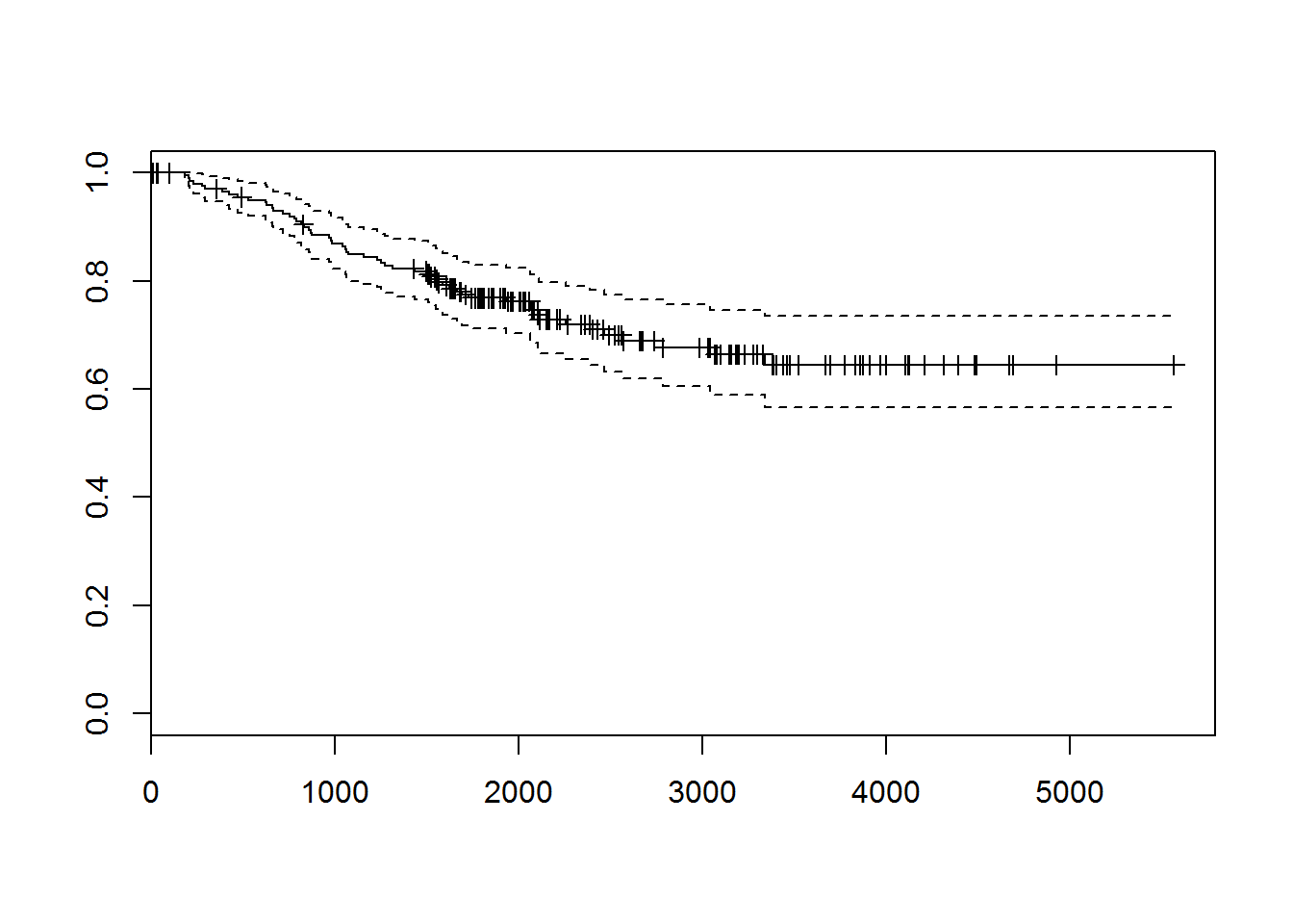
##   [1] 1 0 0 1 1 1 1 1 1 1 1 0 1 1 1 1 1 1 1 1 1 1 1 1 1 0 1 1 1 1 0 1 0 1 1
##  [36] 1 1 1 0 1 1 1 1 0 1 0 1 1 0 0 1 0 0 0 0 1 0 0 0 1 0 0 0 0 0 0 0 0 1 0
##  [71] 0 0 1 0 0 1 0 1 0 0 0 0 1 0 0 0 0 0 1 0 0 1 1 0 1 0 0 1 0 1 1 1 0 0 1
## [106] 0 1 0 0 1 1 1 1 0 0 0 0 0 0 0 0 1 1 0 1 1 1 0 0 1 0 1 1 0 0 0 1 0 1 0
## [141] 1 0 1 0 0 1 0 0 0 0 0 0 0 1 0 0 1 0 0 0 0 1 0 0 1 0 1 1 0 0 1 0 1 1 1
## [176] 0 0 0 0 0 0 1 1 0 0 1 0 0 0 1 1 0 1 1 0 0 0 1 0 0 1 1 0 1 1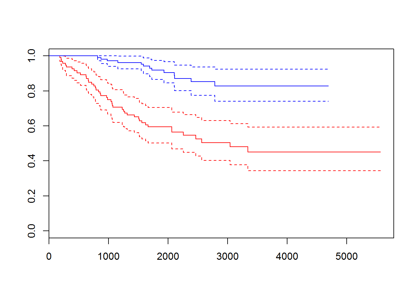
## Call:
## coxph(formula = sData ~ thickness, data = melanoma)
##
##   n= 205, number of events= 57
##
##              coef exp(coef) se(coef)     z Pr(>|z|)
## thickness 0.16024   1.17380  0.03126 5.126 2.96e-07 ***
## ---
## Signif. codes:  0 '***' 0.001 '**' 0.01 '*' 0.05 '.' 0.1 ' ' 1
##
##           exp(coef) exp(-coef) lower .95 upper .95
## thickness     1.174     0.8519     1.104     1.248
##
## Concordance= 0.741  (se = 0.04 )
## Rsquare= 0.089   (max possible= 0.937 )
## Likelihood ratio test= 19.19  on 1 df,   p=1.186e-05
## Wald test            = 26.27  on 1 df,   p=2.964e-07
## Score (logrank) test = 28.7  on 1 df,   p=8.432e-08
## Call:
## coxph(formula = sData ~ age, data = melanoma)
##
## n= 205, number of events= 57
##
## coef exp(coef) se(coef) z Pr(>|z|)
## age 0.019220 1.019406 0.008769 2.192 0.0284 *
## ---
## Signif. codes: 0 '***' 0.001 '**' 0.01 '*' 0.05 '.' 0.1 ' ' 1
##
## exp(coef) exp(-coef) lower .95 upper .95
## age 1.019 0.981 1.002 1.037
##
## Concordance= 0.572 (se = 0.04 )
## Rsquare= 0.024 (max possible= 0.937 )
## Likelihood ratio test= 5 on 1 df, p=0.02534
## Wald test = 4.8 on 1 df, p=0.02839
## Score (logrank) test = 4.83 on 1 df, p=0.02796 ![]()