- Import and Export
Petr V. Nazarov, LIH
2017-05-10
3.1. Current folder
R can import data from local storage or Internet, and export it locally. Let us first setup the current folder, where our results will be stored.
getwd()   # shows current folder
dir()     # shows files in the current folder
setwd("D:/Data/R") # sets the current folder
3.2. Read values from a text file
Here is EUR/USD ratio from January 1999 till April 2017.
We can read values from unformatted text file using scan().
SomeData = scan("http://edu.sablab.net/data/txt/currency.txt",what = "") # what - defines the value class
head(SomeData)
In fact, you can download an entire webpage by scan to parse it afterwards. It’s funny, but we need to get readable data.
3.3. Read tables
We will use read.table() to import the data as a data frame.
| Date | EUR |
|---|---|
| 1999-01-04 | 1.1867 |
| 1999-01-05 | 1.1760 |
| 1999-01-06 | 1.1629 |
| 1999-01-07 | 1.1681 |
| 1999-01-08 | 1.1558 |
Some parameters are important in read.table():
header- set itTRUEif there is a header linesep- separator character."\t"stands for tabulationas.is- prevents transforming character columns to factors.
Currency = read.table("http://edu.sablab.net/data/txt/currency.txt", header=T, sep="\t", as.is=T)
str(Currency)
Do not forget functions that allow you seeing, what is inside your data:
head(Currency)
summary(Currency)
View(Currency)
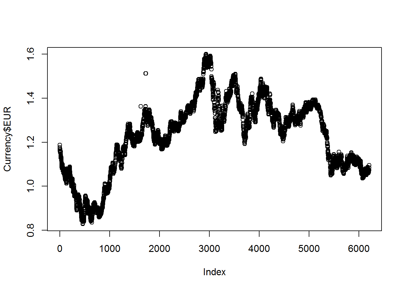
Let’s make the first plot.
plot(Currency$EUR)
Hmm… it’s quite ugly… We will improve it later.
3.4. Read values from binary file
R can keep data in GZip-ed form, automatically loading the variables into memory. Such files have .RData extension. This is a fast & easy way to store your data. Let us first download the data in RData format into you working directory using download.file() and then load it by load(). Parameters of downloading:
destfile- the file name, under which you would like to store the downloaded file.mode- the way you would like to treat the data (as text or binary). To keep binary data unchanged, usewb!
download.file("http://edu.sablab.net/data/all.Rdata",
              destfile="all.Rdata",mode = "wb")

getwd()                # show current folder
dir(pattern=".Rdata")  # show files in the current folder
load("all.RData")      # load the data

ls()                   # you should see 'GE.matrix' among variables

View(GE.matrix)
You can see row and column names of the loaded data.frame object:
attr(GE.matrix,"dimnames")    # annotation of the dimensions
rownames(GE.matrix)
colnames(GE.matrix)
3.5. Data export
There are several ways to export your data. Let’s consider the most simple.
write()- writes a column of numbers / characterswrite.table()- writes a data tablesave()- saves one or several variables into a binary RData file.
Parameters of write.table are:
eol- cheracter for the end of line (can be differ with OS). The standard one is “”dec- decimal separatorquote- do we put “” around character values or notrow.names- do we put row names as a column or not
write.table(Currency,file = "curr.txt",sep = "\t",
            eol = "\n", na = "NA", dec = ".",
            row.names = FALSE, quote=FALSE)

save(Currency,file="Currency.Rdata") # save as binary file

save(list=ls(),file="workspace.Rdata") # save all variables as binary file

getwd()
dir()      # see the results
Exercises
- Dataset from http://edu.sablab.net/data/txt/shop.txt contains records about customers, collected by a women’s apparel store. Check its structure. View its summary.
read.table,View,str,summary,head
- For the “shop” table, save into a new text file only the records for customers, who paid using Visa card.
write.table
