- Desctiptive Statistics
Petr V. Nazarov, LIH
2017-05-10
Let’s load again Mice data:
## clear memory
rm(list = ls())
## load data
Mice=read.table("http://edu.sablab.net/data/txt/mice.txt",header=T,sep="\t")
str(Mice)
## 'data.frame': 790 obs. of 14 variables:
## $ ID : int 1 2 3 368 369 370 371 372 4 5 ...
## $ Strain : Factor w/ 40 levels "129S1/SvImJ",..: 1 1 1 1 1 1 1 1 1 1 ...
## $ Sex : Factor w/ 2 levels "f","m": 1 1 1 1 1 1 1 1 1 1 ...
## $ Starting.age : int 66 66 66 72 72 72 72 72 66 66 ...
## $ Ending.age : int 116 116 108 114 115 116 119 122 109 112 ...
## $ Starting.weight : num 19.3 19.1 17.9 18.3 20.2 18.8 19.4 18.3 17.2 19.7 ...
## $ Ending.weight : num 20.5 20.8 19.8 21 21.9 22.1 21.3 20.1 18.9 21.3 ...
## $ Weight.change : num 1.06 1.09 1.11 1.15 1.08 ...
## $ Bleeding.time : int 64 78 90 65 55 NA 49 73 41 129 ...
## $ Ionized.Ca.in.blood : num 1.2 1.15 1.16 1.26 1.23 1.21 1.24 1.17 1.25 1.14 ...
## $ Blood.pH : num 7.24 7.27 7.26 7.22 7.3 7.28 7.24 7.19 7.29 7.22 ...
## $ Bone.mineral.density: num 0.0605 0.0553 0.0546 0.0599 0.0623 0.0626 0.0632 0.0592 0.0513 0.0501 ...
## $ Lean.tissues.weight : num 14.5 13.9 13.8 15.4 15.6 16.4 16.6 16 14 16.3 ...
## $ Fat.weight : num 4.4 4.4 2.9 4.2 4.3 4.3 5.4 4.1 3.2 5.2 ...6.1. Measures of the center
summary(Mice)## ID Strain Sex Starting.age
## Min. : 1.0 C57BR/cdJ : 28 f:396 Min. :46.00
## 1st Qu.: 310.2 MA/MyJ : 23 m:394 1st Qu.:64.00
## Median : 537.5 CAST/EiJ : 21 Median :66.00
## Mean : 526.8 A/J : 20 Mean :66.21
## 3rd Qu.: 799.8 BTBR_T+_tf/J: 20 3rd Qu.:71.00
## Max. :1012.0 C3H/HeJ : 20 Max. :82.00
## (Other) :658
## Ending.age Starting.weight Ending.weight Weight.change
## Min. : 93.0 Min. : 8.70 Min. :10.00 Min. :0.000
## 1st Qu.:109.0 1st Qu.:17.20 1st Qu.:18.80 1st Qu.:1.059
## Median :114.0 Median :21.20 Median :23.50 Median :1.105
## Mean :114.3 Mean :21.38 Mean :23.69 Mean :1.107
## 3rd Qu.:119.0 3rd Qu.:25.38 3rd Qu.:28.10 3rd Qu.:1.164
## Max. :140.0 Max. :39.10 Max. :49.60 Max. :2.109
## NA's :2
## Bleeding.time Ionized.Ca.in.blood Blood.pH Bone.mineral.density
## Min. : 14 Min. :1.000 Min. :6.810 Min. :0.03980
## 1st Qu.: 43 1st Qu.:1.200 1st Qu.:7.160 1st Qu.:0.04860
## Median : 55 Median :1.240 Median :7.200 Median :0.05300
## Mean : 61 Mean :1.237 Mean :7.199 Mean :0.05331
## 3rd Qu.: 73 3rd Qu.:1.280 3rd Qu.:7.250 3rd Qu.:0.05785
## Max. :522 Max. :1.410 Max. :7.430 Max. :0.07140
## NA's :30 NA's :2 NA's :2 NA's :3
## Lean.tissues.weight Fat.weight
## Min. : 7.30 Min. : 1.800
## 1st Qu.:13.80 1st Qu.: 3.500
## Median :17.30 Median : 4.800
## Mean :17.27 Mean : 6.073
## 3rd Qu.:20.85 3rd Qu.: 7.500
## Max. :29.90 Max. :23.300
## NA's :3 NA's :3## mean and median. We should exclude NA from consideration
mn = mean(Mice$Ending.weight, na.rm=T)
md = median(Mice$Ending.weight, na.rm=T)
## for mode you should add a library:
library(modeest)##
## This is package 'modeest' written by P. PONCET.
## For a complete list of functions, use 'library(help = "modeest")' or 'help.start()'.mo = mlv(Mice$Ending.weight, method = "shorth")$M
## let us plot them
plot(density(Mice$Ending.weight, na.rm=T),lwd=2,main="Ending weight")
abline(v = mn,col="red")
abline(v = md,col="blue")
abline(v = mo ,col="cyan")
legend(x="topright",c("mean","median","mode"),col=c("red","blue","cyan"),pch=19)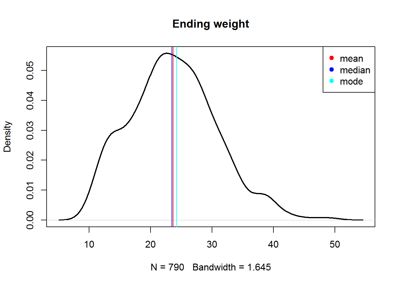
6.2. Measures of variation
## quantiles, percentiles and quartiles
quantile(Mice$Bleeding.time,prob=c(0.25,0.5,0.75),na.rm=T)
## 25% 50% 75%
## 43 55 73## standard deviation and variance
sd(Mice$Bleeding.time, na.rm=T)## [1] 31.91943var(Mice$Bleeding.time, na.rm=T)## [1] 1018.85## stable measure of variation - MAD
mad(Mice$Bleeding.time, na.rm=T)## [1] 20.7564mad(Mice$Bleeding.time, constant = 1, na.rm=T)## [1] 14S6.3. Measures of dependency
## covariation
cov(Mice$Starting.weight,Mice$Ending.weight)
## [1] 39.84946## correlation
cor(Mice$Starting.weight,Mice$Ending.weight)## [1] 0.9422581## coefficient of determination, R2
cor(Mice$Starting.weight,Mice$Ending.weight)^2## [1] 0.8878503## kendal correlation
cor(Mice$Starting.weight,Mice$Ending.weight,method="kendal")## [1] 0.8188964## spearman correlation
cor(Mice$Starting.weight,Mice$Ending.weight,method="spearman")## [1] 0.9423666Excercises.
- Use mice dataset. Calculate the number of mice with bleeding time bigger than 2 minutes
read.table,sumb. Report a 5-numer summary for each column of “mice” data
summary
- For dataset “mice” replace starting weight of any mouse by 1000 (assume, there is a mistype). Calculate mean, median, standard deviation and median absolute deviation (MAD) of this weight. Compare the results with original measures.
mean,median,sd,mad
![]()