- Linar Models
Petr V. Nazarov, LIH
2017-05-10
8.1. ANOVA - analysis of varience
Please see lecture for explanations about ANOVA.
As part of a long-term study of individuals 65 years of age or older, sociologists and physicians at the Wentworth Medical Center in upstate New York investigated the relationship between geographic location and depression. A sample of 60 individuals, all in reasonably good health, and 60 in bad health was selected; 20 individuals were residents of Florida, 20 were residents of New York, and 20 were residents of North Carolina. Each of the individuals sampled was given a standardized test to measure depression. The data collected follow; higher test scores indicate higher levels of depression.
## load data
Data = read.table("http://edu.sablab.net/data/txt/depression2.txt",header=T,sep="\t")
str(Data)
## 'data.frame': 120 obs. of 3 variables:
## $ Location : Factor w/ 3 levels "Florida","New York",..: 1 1 1 1 1 1 1 1 1 1 ...
## $ Health : Factor w/ 2 levels "bad","good": 2 2 2 2 2 2 2 2 2 2 ...
## $ Depression: int 3 7 7 3 8 8 8 5 5 2 ...8.1.1. One-way ANOVA
Let’s take good health people first and see the effect of the location.
DataGH = Data[Data$Health == "good",]

## build 1-factor ANOVA model
res1 = aov(Depression ~  Location, DataGH)
summary(res1)
## Df Sum Sq Mean Sq F value Pr(>F)
## Location 2 78.5 39.27 6.773 0.0023 **
## Residuals 57 330.4 5.80
## ---
## Signif. codes: 0 '***' 0.001 '**' 0.01 '*' 0.05 '.' 0.1 ' ' 18.1.2. Two-way ANOVA
Now, let’s use all data, including bad health respondents.
res2 = aov(Depression ~  Location + Health + Location*Health, data = Data)

## show the ANOVA table
summary(res2)
## Df Sum Sq Mean Sq F value Pr(>F)
## Location 2 73.8 36.9 4.290 0.016 *
## Health 1 1748.0 1748.0 203.094 <2e-16 ***
## Location:Health 2 26.1 13.1 1.517 0.224
## Residuals 114 981.2 8.6
## ---
## Signif. codes: 0 '***' 0.001 '**' 0.01 '*' 0.05 '.' 0.1 ' ' 1We can remove interactions (assume that the effects are purely additive)
res2ni = aov(Depression ~  Location + Health, data = Data)
summary(res2ni)
## Df Sum Sq Mean Sq F value Pr(>F)
## Location 2 73.8 36.9 4.252 0.0165 *
## Health 1 1748.0 1748.0 201.299 <2e-16 ***
## Residuals 116 1007.3 8.7
## ---
## Signif. codes: 0 '***' 0.001 '**' 0.01 '*' 0.05 '.' 0.1 ' ' 1Some examples of reporting the importance:
## get p-values
pv=(summary(res2)[[1]][,5])
names(pv) = rownames(summary(res2)[[1]])
barplot(-log(pv),ylab="-log10(p-value)")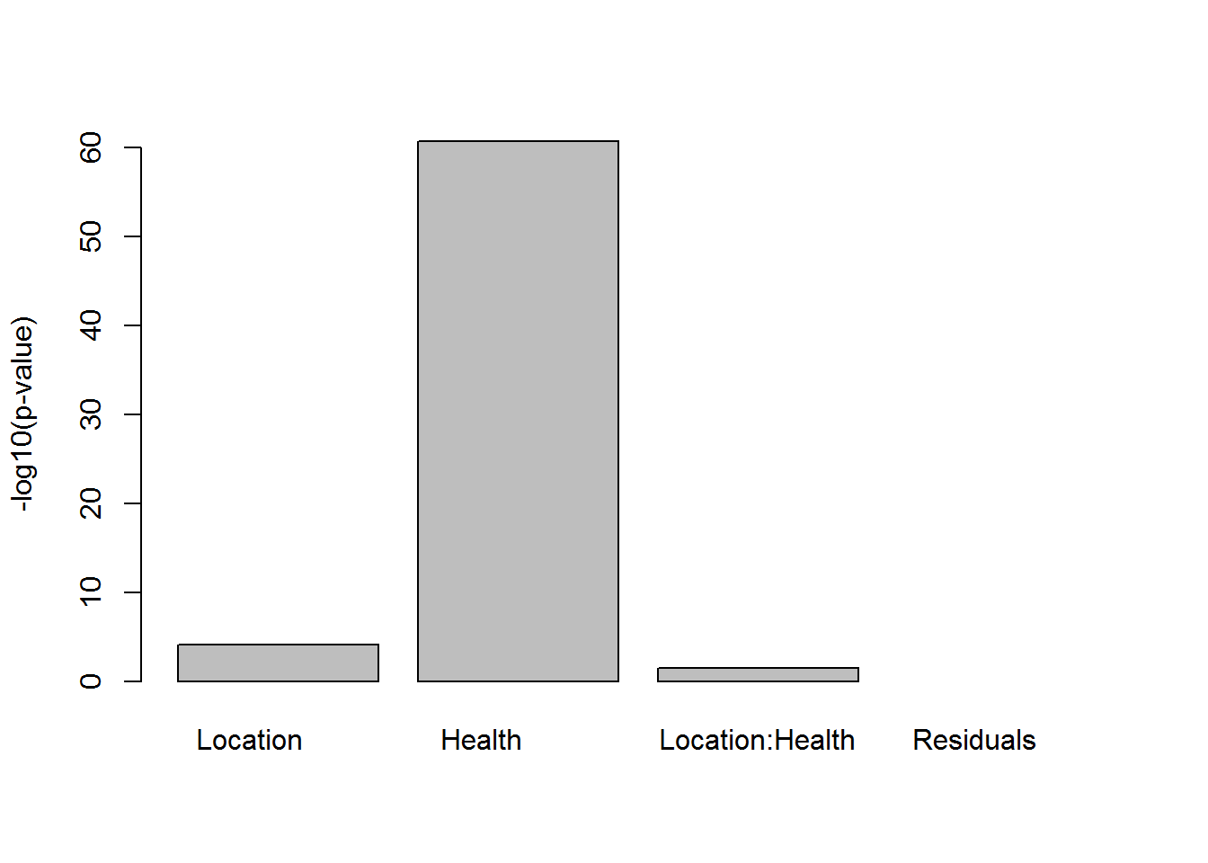
8.1.3. Post-hoc analysis
TukeyHSD(res1)## Tukey multiple comparisons of means
## 95% family-wise confidence level
##
## Fit: aov(formula = Depression ~ Location, data = DataGH)
##
## $Location
## diff lwr upr p adj
## New York-Florida 2.8 0.9677423 4.6322577 0.0014973
## North Carolina-Florida 1.5 -0.3322577 3.3322577 0.1289579
## North Carolina-New York -1.3 -3.1322577 0.5322577 0.2112612TukeyHSD(res2)## Tukey multiple comparisons of means
## 95% family-wise confidence level
##
## Fit: aov(formula = Depression ~ Location + Health + Location * Health, data = Data)
##
## $Location
## diff lwr upr p adj
## New York-Florida 1.850 0.2921599 3.4078401 0.0155179
## North Carolina-Florida 0.475 -1.0828401 2.0328401 0.7497611
## North Carolina-New York -1.375 -2.9328401 0.1828401 0.0951631
##
## $Health
## diff lwr upr p adj
## good-bad -7.633333 -8.694414 -6.572252 0
##
## $`Location:Health`
## diff lwr upr
## New York:bad-Florida:bad 0.90 -1.7893115 3.589311
## North Carolina:bad-Florida:bad -0.55 -3.2393115 2.139311
## Florida:good-Florida:bad -8.95 -11.6393115 -6.260689
## New York:good-Florida:bad -6.15 -8.8393115 -3.460689
## North Carolina:good-Florida:bad -7.45 -10.1393115 -4.760689
## North Carolina:bad-New York:bad -1.45 -4.1393115 1.239311
## Florida:good-New York:bad -9.85 -12.5393115 -7.160689
## New York:good-New York:bad -7.05 -9.7393115 -4.360689
## North Carolina:good-New York:bad -8.35 -11.0393115 -5.660689
## Florida:good-North Carolina:bad -8.40 -11.0893115 -5.710689
## New York:good-North Carolina:bad -5.60 -8.2893115 -2.910689
## North Carolina:good-North Carolina:bad -6.90 -9.5893115 -4.210689
## New York:good-Florida:good 2.80 0.1106885 5.489311
## North Carolina:good-Florida:good 1.50 -1.1893115 4.189311
## North Carolina:good-New York:good -1.30 -3.9893115 1.389311
## p adj
## New York:bad-Florida:bad 0.9264595
## North Carolina:bad-Florida:bad 0.9913348
## Florida:good-Florida:bad 0.0000000
## New York:good-Florida:bad 0.0000000
## North Carolina:good-Florida:bad 0.0000000
## North Carolina:bad-New York:bad 0.6244461
## Florida:good-New York:bad 0.0000000
## New York:good-New York:bad 0.0000000
## North Carolina:good-New York:bad 0.0000000
## Florida:good-North Carolina:bad 0.0000000
## New York:good-North Carolina:bad 0.0000003
## North Carolina:good-North Carolina:bad 0.0000000
## New York:good-Florida:good 0.0361494
## North Carolina:good-Florida:good 0.5892328
## North Carolina:good-New York:good 0.7262066TukeyHSD(res2ni)## Tukey multiple comparisons of means
## 95% family-wise confidence level
##
## Fit: aov(formula = Depression ~ Location + Health, data = Data)
##
## $Location
## diff lwr upr p adj
## New York-Florida 1.850 0.2855861 3.4144139 0.0160324
## North Carolina-Florida 0.475 -1.0894139 2.0394139 0.7516558
## North Carolina-New York -1.375 -2.9394139 0.1894139 0.0970280
##
## $Health
## diff lwr upr p adj
## good-bad -7.633333 -8.698937 -6.567729 08.2. Linear regression
Example. Cells are grown under different temperature conditions from \(20^\circ\) to \(40^\circ\). A researched would like to find a dependency between T and cell number. Let us build a linear regression:
Data = read.table("http://edu.sablab.net/data/txt/cells.txt", header=T,sep="\t",quote="\"")
x = Data$Temperature
y = Data$Cell.Number
res = lm(y~x)
res
##
## Call:
## lm(formula = y ~ x)
##
## Coefficients:
## (Intercept) x
## -190.78 15.33summary(res)##
## Call:
## lm(formula = y ~ x)
##
## Residuals:
## Min 1Q Median 3Q Max
## -49.183 -26.190 -1.185 22.147 54.477
##
## Coefficients:
## Estimate Std. Error t value Pr(>|t|)
## (Intercept) -190.784 35.032 -5.446 2.96e-05 ***
## x 15.332 1.145 13.395 3.96e-11 ***
## ---
## Signif. codes: 0 '***' 0.001 '**' 0.01 '*' 0.05 '.' 0.1 ' ' 1
##
## Residual standard error: 31.76 on 19 degrees of freedom
## Multiple R-squared: 0.9042, Adjusted R-squared: 0.8992
## F-statistic: 179.4 on 1 and 19 DF, p-value: 3.958e-11…and visualize it with condifence and predictions intervals (see lecture for the details)
# draw the data
plot(x,y)
# draw the regression and its confidence (95%)
lines(x, predict(res,int = "confidence")[,1],col=4,lwd=2)
lines(x, predict(res,int = "confidence")[,2],col=4)
lines(x, predict(res,int = "confidence")[,3],col=4)
# draw the prediction for the values (95%)
lines(x, predict(res,int = "pred")[,2],col=2)
## Warning in predict.lm(res, int = "pred"): predictions on current data refer to _future_ responseslines(x, predict(res,int = "pred")[,3],col=2)## Warning in predict.lm(res, int = "pred"): predictions on current data refer to _future_ responses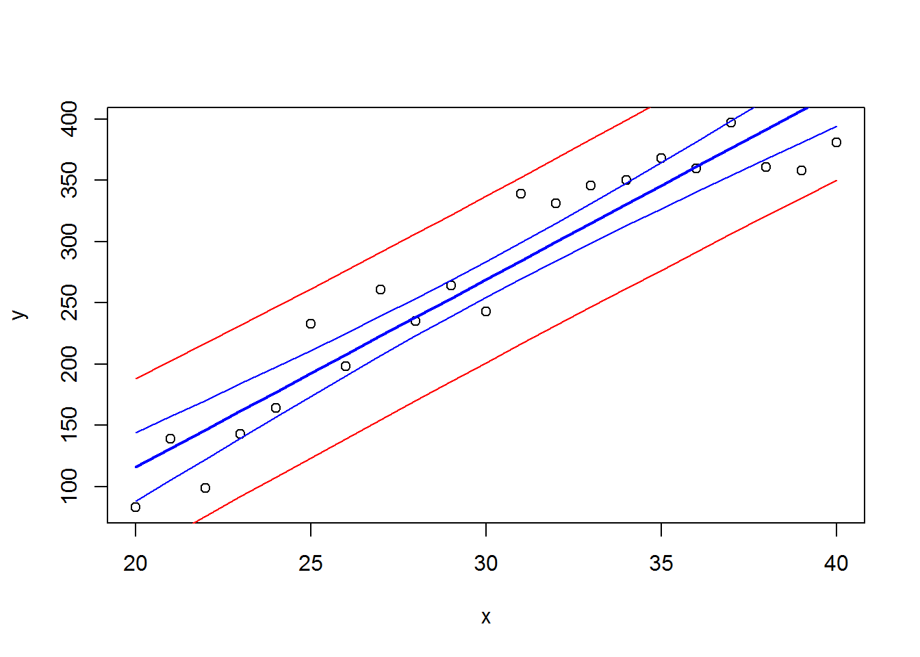
- Data set teeth contains the result of an experiment, conducted to measure the effect of various doses of vitamin C on the tooth growth (model animal – Guinea pigs). Vitamin C and orange juice were given to animals in different quantities. Using 2-way ANOVA study the effects of vitamin-C and orange juice.
aov,summary
- Work with mice data from http://edu.sablab.net/data/txt/mice.txt . Study the effects of sex and strain on mouse weight and other parameters.
aov, summary
- A biology student wishes to determine the relationship between temperature and heart rate in leopard frog, Rana pipiens. He manipulates the temperature in 2o increment ranging from 2 to 18 o C and records the heart rate at each interval. His data are presented in table rana.txt
- Build the model and provide the p-value for linear dependency
- Provide interval estimation for the slope of the dependency
- Estimate 95% prediction interval for heart rate at 15
lm,summary,predict,confint
- Data are stored in this dataset for two groups of patients who died of acute myelogenous leukemia. Patients were classified into the two groups according to the presence or absence of a morphologic characteristic of white cells. Patients termed AG positive were identified by the presence of Auer rods and/or significant granulature of the leukemic cells in the bone marrow at diagnosis. For AG-negative patients, these factors were absent. Leukemia is a cancer characterized by an overproliferation of white blood cells; the higher the white blood count (WBC), the more severe the disease. Separately for each morphologic group, AG positive and AG negative perform regression analysis of WBC-survival dependency. Consider log-transform the data if necessary.
lm,summary,log
![]()