- Clustering and PCA
Petr V. Nazarov, LIH
2017-05-10
9.1. PCA - principal component analysis
9.1.1. PCA of iris data
## show the data
str(iris)
## 'data.frame': 150 obs. of 5 variables:
## $ Sepal.Length: num 5.1 4.9 4.7 4.6 5 5.4 4.6 5 4.4 4.9 ...
## $ Sepal.Width : num 3.5 3 3.2 3.1 3.6 3.9 3.4 3.4 2.9 3.1 ...
## $ Petal.Length: num 1.4 1.4 1.3 1.5 1.4 1.7 1.4 1.5 1.4 1.5 ...
## $ Petal.Width : num 0.2 0.2 0.2 0.2 0.2 0.4 0.3 0.2 0.2 0.1 ...
## $ Species : Factor w/ 3 levels "setosa","versicolor",..: 1 1 1 1 1 1 1 1 1 1 ...## plot it
plot(iris[,-5],col = iris[,5],pch=19)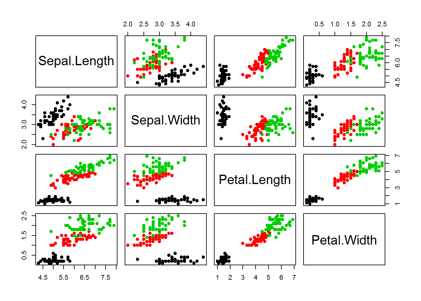
# transform data frame to a matrix
iX = as.matrix(iris[,-5])
row.names(iX) = as.character(iris[,5])
classes = as.integer(iris[,5])

## perform PCA. We need data to be a matrix
PC = prcomp(iX)
str(PC)
## List of 5
## $ sdev : num [1:4] 2.056 0.493 0.28 0.154
## $ rotation: num [1:4, 1:4] 0.3614 -0.0845 0.8567 0.3583 -0.6566 ...
## ..- attr(*, "dimnames")=List of 2
## .. ..$ : chr [1:4] "Sepal.Length" "Sepal.Width" "Petal.Length" "Petal.Width"
## .. ..$ : chr [1:4] "PC1" "PC2" "PC3" "PC4"
## $ center : Named num [1:4] 5.84 3.06 3.76 1.2
## ..- attr(*, "names")= chr [1:4] "Sepal.Length" "Sepal.Width" "Petal.Length" "Petal.Width"
## $ scale : logi FALSE
## $ x : num [1:150, 1:4] -2.68 -2.71 -2.89 -2.75 -2.73 ...
## ..- attr(*, "dimnames")=List of 2
## .. ..$ : chr [1:150] "setosa" "setosa" "setosa" "setosa" ...
## .. ..$ : chr [1:4] "PC1" "PC2" "PC3" "PC4"
## - attr(*, "class")= chr "prcomp"## plot PC1 and PC2 only
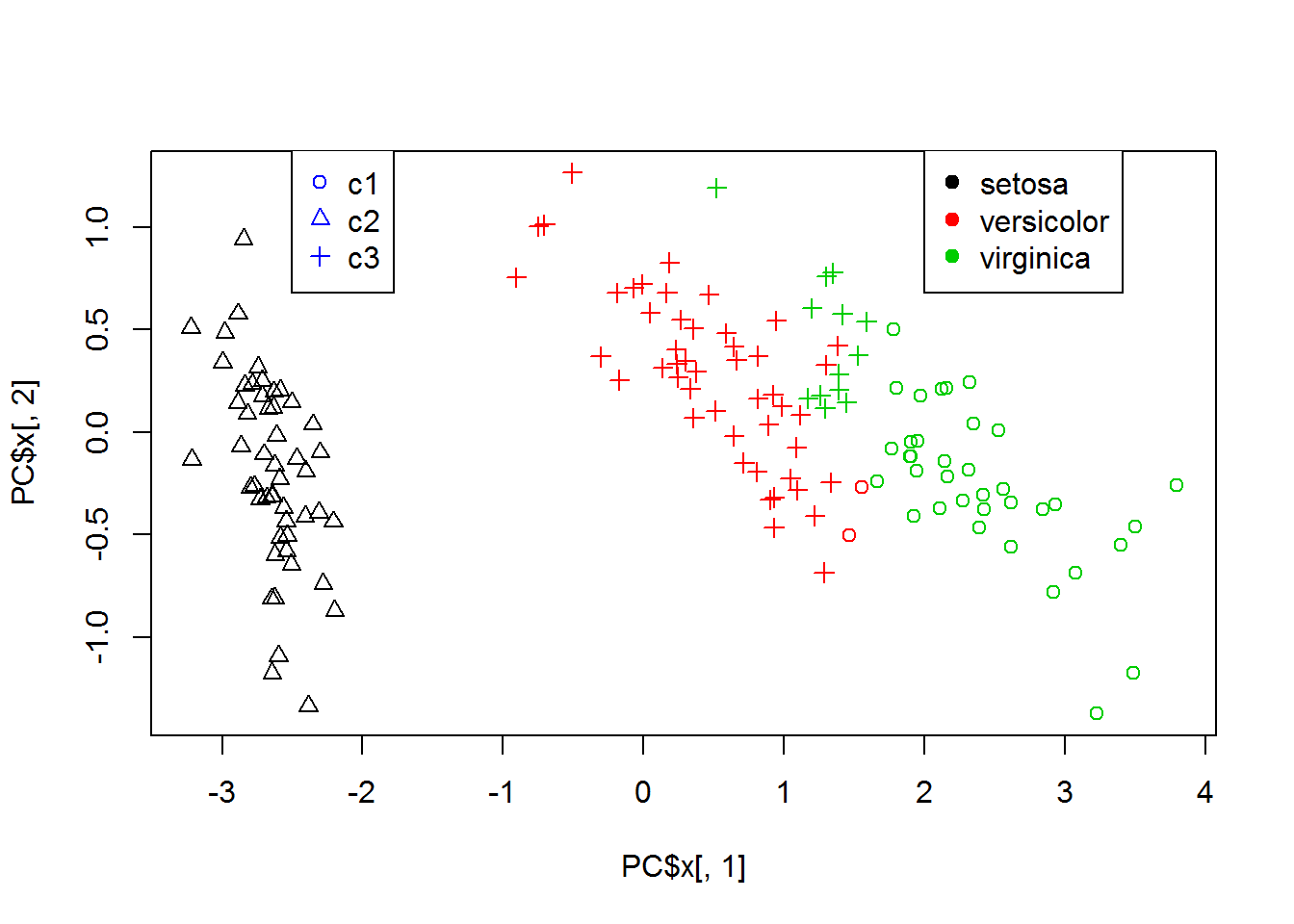
plot(PC$x[,1],PC$x[,2], col=classes, pch=19)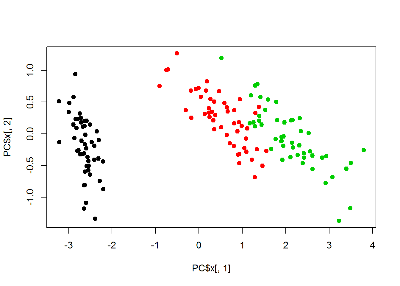
You can use 3D visualization:
library(rgl)
plot3d(PC$x[,1],PC$x[,2],PC$x[,3],
       size = 2,
       col  = classes,
       type = "s",
       xlab = "PC1",
       ylab = "PC2",
       zlab = "PC3")
9.1.2 PCA for Mice
Mice = read.table("http://edu.sablab.net/data/txt/mice.txt",header=T,sep="\t")
Data = as.matrix(Mice[,-(1:5)])
Data[is.na(Data)] = 0
PC = prcomp(Data,scale=TRUE)
## TRUE - will capture technical outliers (absent values)
## FALSE - will capture mailny bleding time (highest values)

str(PC)
## List of 5
## $ sdev : num [1:9] 2.005 1.322 1.004 0.966 0.754 ...
## $ rotation: num [1:9, 1:9] 0.4393 0.4652 0.1787 -0.0666 0.2121 ...
## ..- attr(*, "dimnames")=List of 2
## .. ..$ : chr [1:9] "Starting.weight" "Ending.weight" "Weight.change" "Bleeding.time" ...
## .. ..$ : chr [1:9] "PC1" "PC2" "PC3" "PC4" ...
## $ center : Named num [1:9] 21.38 23.69 1.11 58.68 1.23 ...
## ..- attr(*, "names")= chr [1:9] "Starting.weight" "Ending.weight" "Weight.change" "Bleeding.time" ...
## $ scale : Named num [1:9] 5.9834 7.0682 0.1124 33.4098 0.0879 ...
## ..- attr(*, "names")= chr [1:9] "Starting.weight" "Ending.weight" "Weight.change" "Bleeding.time" ...
## $ x : num [1:790, 1:9] -0.596 -0.977 -1.313 -0.33 -0.109 ...
## ..- attr(*, "dimnames")=List of 2
## .. ..$ : NULL
## .. ..$ : chr [1:9] "PC1" "PC2" "PC3" "PC4" ...
## - attr(*, "class")= chr "prcomp"## plot PC1 and PC2 only
col=c("#AA002255","#0000AA55")
plot(PC$x[,1],PC$x[,2],col=col[Mice$Sex], pch=19)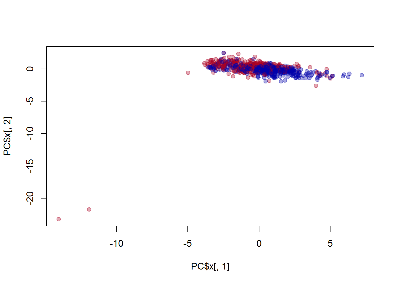
text(PC$x[,1],PC$x[,2]-0.5,Mice$ID,cex=0.6,col="#000000AA")

## investigate manually the outliers
Mice[Mice$ID == 927,]
Mice[Mice$ID == 169,]
9.1.3 PCA for ALL
ALL = read.table("http://edu.sablab.net/data/txt/all_data.txt",as.is=T,header=T,sep="\t")
head(ALL) ## see here - experiments are in columns!!!
## ID Name ALL_GSM51674 ALL_GSM51675
## 1 A1BG alpha-1-B glycoprotein 5.172020 5.362170
## 2 A1CF APOBEC1 complementation factor 6.161910 6.010830
## 3 A2BP1 ataxin 2-binding protein 1 6.892650 6.420090
## 4 A2LD1 AIG2-like domain 1 5.823875 5.807825
## 5 A2M alpha-2-macroglobulin 6.104955 6.136995
## 6 A2ML1 alpha-2-macroglobulin-like 1 5.130645 5.009005
## ALL_GSM51676 ALL_GSM51677 ALL_GSM51678 ALL_GSM51679 ALL_GSM51680
## 1 5.423010 5.229340 5.630930 5.298720 5.724870
## 2 5.754380 6.120220 6.572630 5.683060 5.947680
## 3 6.744630 6.071700 6.583860 6.442820 6.523570
## 4 5.522770 5.601265 5.658775 5.842810 5.813395
## 5 6.159920 6.098240 6.340465 5.877555 6.053760
## 6 4.861405 5.041615 5.161135 4.979330 4.969580
## ALL_GSM51681 ALL_GSM51682 ALL_GSM51683 ALL_GSM51684 ALL_GSM51685
## 1 5.327440 5.369400 5.796450 5.576530 6.319930
## 2 5.926130 5.780850 5.128680 5.841330 7.133310
## 3 6.582650 5.900120 6.157160 6.361310 7.076060
## 4 5.881180 5.701905 5.694900 5.551300 6.178565
## 5 5.707530 5.910775 5.596555 6.187125 6.646705
## 6 4.674275 4.964315 4.682130 4.988795 5.624545
## ALL_GSM51686 ALL_GSM51687 ALL_GSM51688 ALL_GSM51689 ALL_GSM51690
## 1 5.849260 5.929620 5.341570 5.738520 6.918840
## 2 6.900400 7.146370 7.983990 7.998680 5.299670
## 3 7.593170 7.440910 8.019550 7.890730 6.898070
## 4 6.577855 6.410115 6.885735 6.820155 5.516975
## 5 6.912990 6.735105 7.130255 6.706005 5.899060
## 6 5.576735 5.436000 5.779315 6.077210 4.947345
## ALL_GSM51691 ALL_GSM51692 ALL_GSM51693 ALL_GSM51694 ALL_GSM51695
## 1 6.11562 6.988130 6.064130 6.16315 6.095410
## 2 5.26327 5.815450 5.279250 5.62446 5.332180
## 3 5.83715 6.131690 5.925890 6.27410 5.750980
## 4 5.42296 5.693785 5.517325 4.89489 5.377655
## 5 5.64484 5.321100 5.683065 5.82829 5.799450
## 6 4.75725 5.375030 4.787830 4.84364 4.821295
## ALL_GSM51696 ALL_GSM51697 ALL_GSM51698 ALL_GSM51699 ALL_GSM51700
## 1 6.306610 6.066170 6.211270 6.86911 6.615320
## 2 4.982410 5.276320 5.017690 5.62981 5.425400
## 3 6.096900 5.934490 5.813880 6.35552 5.872480
## 4 4.712980 5.206705 5.049215 5.38947 4.789460
## 5 5.933815 5.928810 5.801360 5.71199 5.578660
## 6 4.864400 4.737280 4.718120 4.71069 4.926445
## ALL_GSM51701 ALL_GSM51702 ALL_GSM51703 ALL_GSM51704 ALL_GSM51705
## 1 6.775450 7.010850 6.187840 6.292000 6.745140
## 2 5.684650 4.909680 5.167770 5.260720 5.268680
## 3 6.200590 6.080080 5.827720 5.826990 5.625660
## 4 5.271440 5.414530 5.415650 5.192020 5.365275
## 5 5.685550 7.018595 6.410230 6.679415 6.601430
## 6 4.873015 4.967425 4.613165 4.690265 4.754480
## ALL_GSM51706 ALL_GSM51707 ALL_GSM51708 ALL_GSM51709 ALL_GSM51710
## 1 6.382470 6.458090 6.167130 6.288490 6.983540
## 2 5.215880 5.837160 5.122080 5.461310 5.020010
## 3 5.775370 6.513040 6.148690 6.051390 6.067970
## 4 5.358295 5.351890 5.488120 5.580700 5.910510
## 5 6.429480 6.262625 5.718955 5.665425 5.853005
## 6 4.733625 4.905855 4.787905 4.766025 4.564565
## ALL_GSM51711 ALL_GSM51712 normal_GSM270834 normal_GSM270835
## 1 6.453630 6.561750 6.219560 6.497950
## 2 4.887170 5.308550 5.259040 5.008200
## 3 5.791470 5.896220 6.089660 5.977700
## 4 5.791790 5.486475 5.583065 5.458360
## 5 5.768930 5.760060 5.803010 5.751760
## 6 4.986665 4.784090 4.758815 4.766945
## normal_GSM270836 normal_GSM270837 normal_GSM270838 normal_GSM270839
## 1 6.207010 6.44843 5.667910 6.584080
## 2 4.956770 5.19183 5.501120 5.704030
## 3 6.185220 6.14886 6.442940 5.954080
## 4 5.387995 5.63607 5.614045 5.204815
## 5 5.735520 5.70869 6.535770 6.017905
## 6 4.809925 4.69613 4.935185 4.666620
## normal_GSM270840 normal_GSM270841 normal_GSM270842 normal_GSM270843
## 1 6.98373 6.916530 6.774840 6.741230
## 2 5.08589 5.484820 4.979650 5.343280
## 3 6.06854 5.708460 5.949640 6.223840
## 4 5.23499 5.434170 5.436440 5.603940
## 5 5.84826 5.663120 5.709140 5.630935
## 6 4.77154 4.937805 4.927015 4.771795
## normal_GSM270844 normal_GSM50698 normal_GSM50699 normal_GSM50700
## 1 7.317240 7.052560 6.910190 6.540540
## 2 5.620210 5.377420 5.651280 4.859890
## 3 6.177330 6.057150 5.925810 6.152210
## 4 5.263115 5.269520 5.053050 5.674920
## 5 5.675910 5.673955 5.874995 5.708425
## 6 4.968940 4.646460 4.971815 4.941655
## normal_GSM50701 normal_GSM50702
## 1 6.284930 6.624860
## 2 5.897410 5.390920
## 3 5.866840 6.280300
## 4 5.723595 5.846535
## 5 5.356915 5.717825
## 6 4.741810 4.792475## Transform to matrix
Data=as.matrix(ALL[,-(1:2)])
## assign colors based on column names
color = colnames(Data)
color[grep("ALL",color)]="red"
color[grep("normal",color)]="blue"
## perform PCA (on transposed matrix!)
PC = prcomp(t(Data))
## plot PC1 and PC2 only
plot(PC$x[,1],PC$x[,2],col=color,pch=19,cex=2)
text(PC$x[,1],PC$x[,2]+5,colnames(Data),cex=0.6)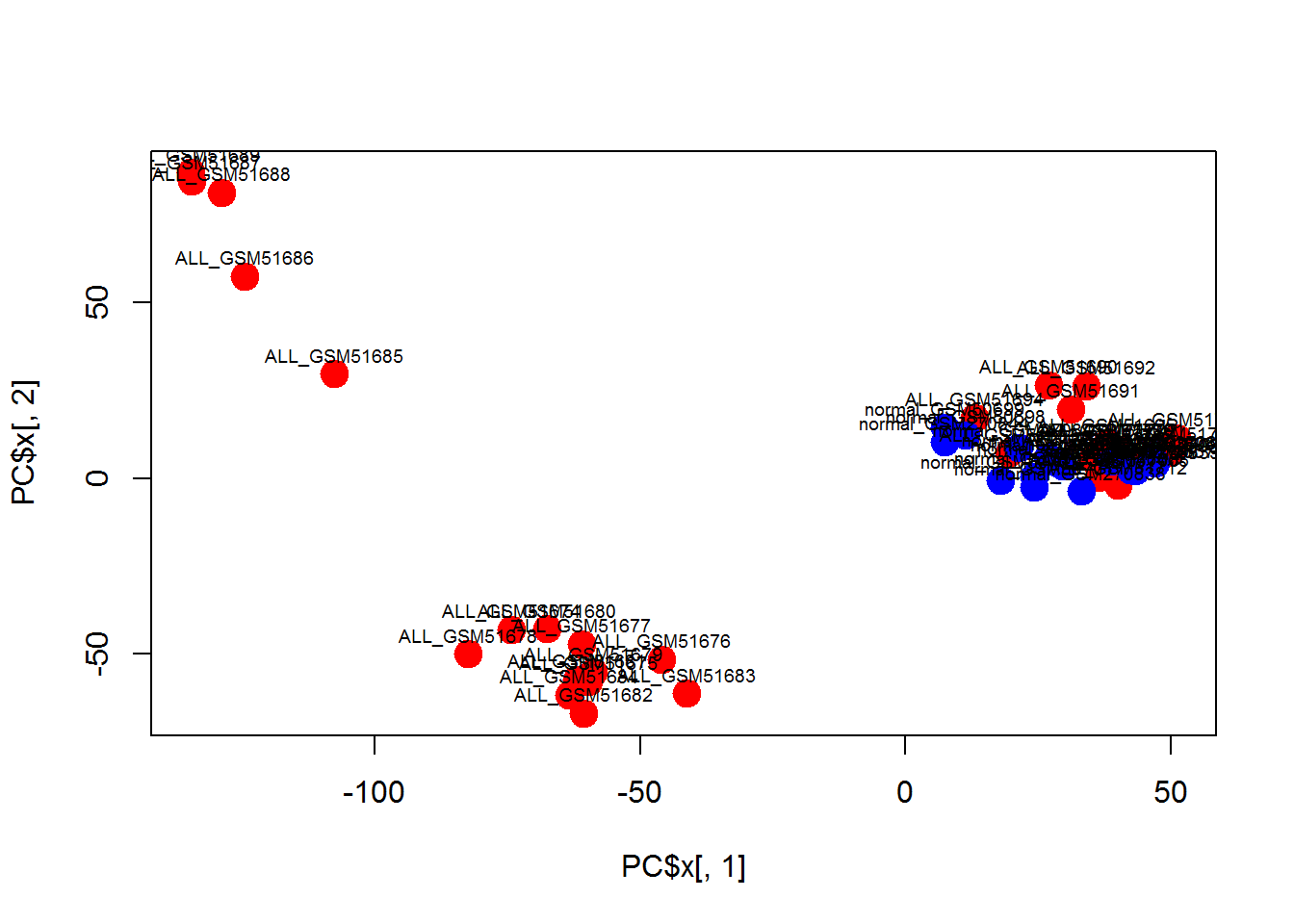
9.2. Clustering
9.2.1. k-means
k-means is a fast and robust clustering method. Main problem - not flexible :)
# remember 'iris' dataset ?
str(iX)
## num [1:150, 1:4] 5.1 4.9 4.7 4.6 5 5.4 4.6 5 4.4 4.9 ...
## - attr(*, "dimnames")=List of 2
## ..$ : chr [1:150] "setosa" "setosa" "setosa" "setosa" ...
## ..$ : chr [1:4] "Sepal.Length" "Sepal.Width" "Petal.Length" "Petal.Width"# clustring
clusters = kmeans(x=iX,centers=3,nstart=10)$cluster
str(clusters)## Named int [1:150] 2 2 2 2 2 2 2 2 2 2 ...
## - attr(*, "names")= chr [1:150] "setosa" "setosa" "setosa" "setosa" ...# rerun PCA
PC = prcomp(iX)
{
plot(PC$x[,1],PC$x[,2],col = classes,pch=clusters)
legend(2,1.4,levels(iris$Species),col=c(1,2,3),pch=19)
legend(-2.5,1.4,c("c1","c2","c3"),col=4,pch=c(1,2,3))
}
9.2.3. Heatmaps and hierarchical clustering
When heatmap is built, it automatically performs hiererchical clustering.
## use heatmap with colors
classes = as.integer(iris[,5])
color = character(length(classes))
color[classes == 1] = "black"
color[classes == 2] = "red"
color[classes == 3] = "green"
## modify the heatmap colors
heatmap(t(iX), scale="none",ColSideColors=color,  col = colorRampPalette (c("blue","wheat","red"))(1000))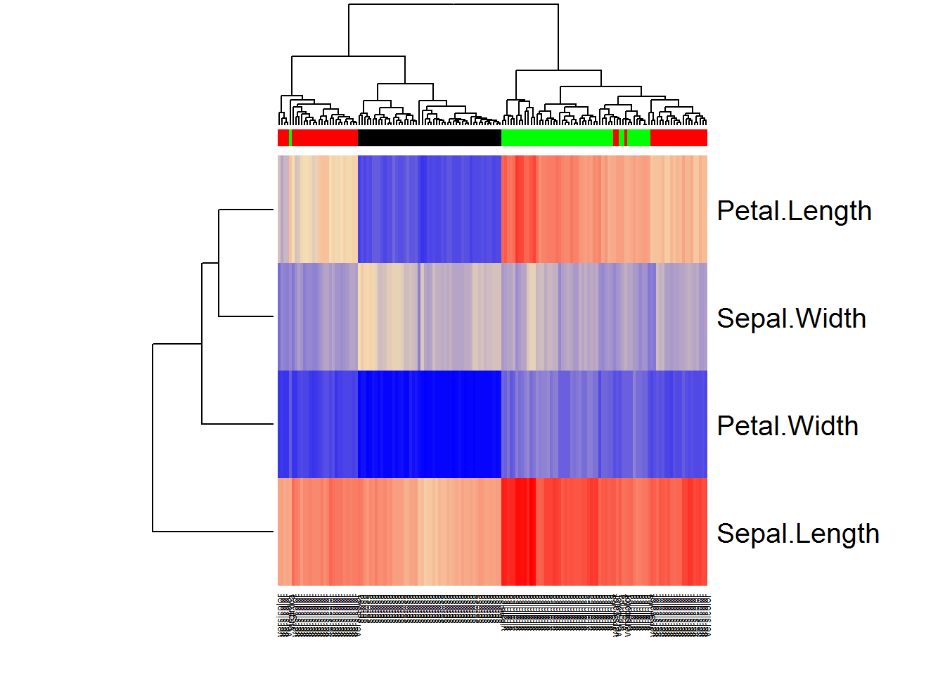
plot(hclust(dist(iX)))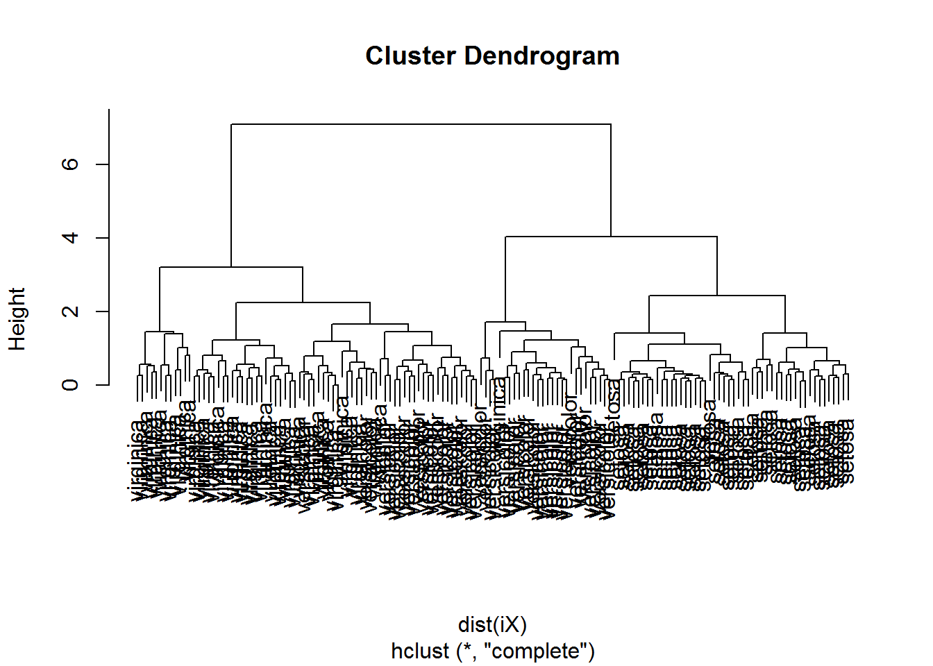
Excercises
- Work with mice data. Perform PCA and identify outliers (or strangely behaving creatures) among mice population. Hint: Replace NA values in each column by the corresponding median value (for this column).
prcomp
- Acute lymphoblastic leukemia (ALL), is a form of leukemia characterized by excess lymphoblasts. ALL contains the results of transcriptome profiling for ALL patients and healthy donors using Affymetrix microarrays. The expression values in the table are in log2 scale. See data http://edu.sablab.net/data/txt/all_data.txt . Perform exploratory analysis of ALL dataset using PCA
prcomp
- Work with ALL dataset. Using t-test, identify top 100 genes with significantly different expression b/w ALL and normal condition. Build a hierarchical clustering for these genes
t.test, heatmap
![]()