- Differential Gene Expression Analysis
Petr V. Nazarov, LIH
2018-03-05
4.0. Installation of the required libraries
In the native R, the vast majority of the libraries (or packages) can be simply installed by install.libraries("library_name"). However, some advanced R/Bioconductor packages may need advanced handling of the dependencies. Thus, we would recomend using biocLite() function:
source("https://bioconductor.org/biocLite.R")

biocLite("limma")
biocLite("edgeR")
biocLite("DESeq2")
4.1. Analysis of microarrays
Here we will consider only modern one-colour arrays. However the methods were developed and are applicable for two-colour arrays.
If you work with Affymetrix (now ThermoFisher) one-colour arrays - be prepared that some preliminary step should be performed before you can really touch the data. Binary CEL files should be processed by one of the tools, probe intensity normalized and summarized into probesets (old arrays and arrays targeted at splicing) or transcript clusters. The later is (to some extent) a synonym for “genes”. Some tools that can help are listed below:
TrancriptomeAnalysis Console (TAC) - free and quite advanced tool. Allows import Affymetrix and Thermofisher (Clariom) arrays, RMA normalizations with GC correction, data visualization, statistical analysis and functional annotation. (strongly recommended for Affy/Thermo arrays)
Affymetrix Power Tools (APT) - free & flexible command line tools for older versions of Affymetrix arrays.
oligo package of R/Bioconductor - free tool for R geeks :). For example of application - see Exercise 6 of AdvBiostat course.
Here we will consider results from TAC software. See 2 files online: HTA.txt contains expression measure by HTA 2.0 arrays and HTA_anno.txt. We consider here only gene-level analysis, thus leaving exon and junction characterization aside.
4.1.1 Data loading
## load data
Data = read.table("http://edu.sablab.net/rt2018/data/HTA.txt",header=T,sep="\t",row.names = 1)
str(Data)
## 'data.frame': 67528 obs. of 18 variables:
## $ ST327_.HTA.2_0..sst.rma.combined.dabg.chp.Signal: num 7.6 6.67 6.14 5.47 5.66 4.66 5.63 5.66 5.4 4.3 ...
## $ SN327_.HTA.2_0..sst.rma.combined.dabg.chp.Signal: num 18.9 17.9 15.3 14.2 14.3 ...
## $ ST328_.HTA.2_0..sst.rma.combined.dabg.chp.Signal: num 7.7 6.76 6.24 5.81 5.85 6.19 6.06 7.23 5.53 4.34 ...
## $ SN328_.HTA.2_0..sst.rma.combined.dabg.chp.Signal: num 18.7 17.7 16.2 15.6 15.5 ...
## $ ST349_.HTA.2_0..sst.rma.combined.dabg.chp.Signal: num 6.91 6.46 6.45 5.81 6.05 5.33 5.63 6.22 5.62 4.25 ...
## $ SN349_.HTA.2_0..sst.rma.combined.dabg.chp.Signal: num 18.7 17.9 17.4 17.2 16.9 ...
## $ ST354_.HTA.2_0..sst.rma.combined.dabg.chp.Signal: num 6.93 6.3 6.41 5.77 6.05 5.66 6.23 5.81 5.45 4.14 ...
## $ SN354_.HTA.2_0..sst.rma.combined.dabg.chp.Signal: num 19.3 18.6 17.9 17.9 17.5 ...
## $ ST405_.HTA.2_0..sst.rma.combined.dabg.chp.Signal: num 7.35 6.59 6.1 5.58 5.74 6.36 5.63 7.53 6.11 4.59 ...
## $ SN405_.HTA.2_0..sst.rma.combined.dabg.chp.Signal: num 19.4 18.7 17.1 16.5 17.2 ...
## $ ST449_.HTA.2_0..sst.rma.combined.dabg.chp.Signal: num 7.37 6.55 6.29 5.68 5.86 4.65 5.75 5.76 5.41 4.75 ...
## $ SN449_.HTA.2_0..sst.rma.combined.dabg.chp.Signal: num 18.9 18 17.4 17.1 16.7 ...
## $ ST450_.HTA.2_0..sst.rma.combined.dabg.chp.Signal: num 7.42 6.95 6.39 5.57 5.56 5.73 5.47 6.62 5.55 4.76 ...
## $ SN450_.HTA.2_0..sst.rma.combined.dabg.chp.Signal: num 18.9 18.2 16.9 16.7 16.3 ...
## $ ST667_.HTA.2_0..sst.rma.combined.dabg.chp.Signal: num 7.62 6.27 6 5.19 5.69 4.81 5.7 5.86 5.25 4.49 ...
## $ SN667_.HTA.2_0..sst.rma.combined.dabg.chp.Signal: num 18.9 17.4 16.6 16.6 15 ...
## $ ST679_.HTA.2_0..sst.rma.combined.dabg.chp.Signal: num 7.1 6.53 6.23 5.42 5.93 4.8 5.71 5.72 5.28 4.51 ...
## $ SN679_.HTA.2_0..sst.rma.combined.dabg.chp.Signal: num 18.6 18.2 16.9 16.7 16.7 ...## load annotation
Anno = read.table("http://edu.sablab.net/rt2018/data/HTA_anno.txt",header=T,sep="\t",row.names = 1, as.is=TRUE)
Anno = Anno[rownames(Data),] ## force the same order
str(Anno)## 'data.frame': 67528 obs. of 8 variables:
## $ Gene.Symbol : chr "PRR4" "PRB3" "PRB4" "PRB4" ...
## $ Public.Gene.IDs: chr "NM_001098538; NM_007244; ENST00000228811; ENST00000540107; ENST00000544994; AK311715; BC058035; uc001qyz.4; uc0"| __truncated__ "NM_006249; ENST00000381842; ENST00000538488; BC096209; uc001qzs.3" "BC128191; K03207" "NM_002723; ENST00000279575; ENST00000445719; ENST00000535904; BC130386" ...
## $ Description : chr "proline rich 4 (lacrimal)" "proline-rich protein BstNI subfamily 3" "proline-rich protein BstNI subfamily 4" "proline-rich protein BstNI subfamily 4" ...
## $ Chromosome : chr "chr12" "chr12" "chr12" "chr12" ...
## $ Strand : chr "-" "-" "-" "-" ...
## $ Group : chr "Coding" "Coding" "NonCoding" "Coding" ...
## $ Start : int 10998448 11418857 11460017 11460015 11504757 142829170 11504757 1151580 1151580 127840600 ...
## $ Stop : int 11002075 11422739 11463369 11463369 11508525 142836839 11508525 1261606 1253774 127912962 ...
4.1.2 limma - LInear Models for MicroArrays
Limma works similar to ANOVA with somewhat improved post-hoc analysis and p-value calculation (empirical Bayes statistics). Let’s first see how to do simple analysis and then consider a warp-up function.
X = as.matrix(Data) ## not really needed... You can work with Data
colnames(X) = sub("_.+","",colnames(X))

library(limma)
## we should create factors
groups = sub("[0-9].+","",colnames(X))
people = sub("[A-Z]+","",colnames(X))
groups = factor(groups)
people = factor(paste0("P",people))

## now create desigh matrix (a lot of FUN !)
design = model.matrix(~ -1 + groups)
colnames(design)=sub("groups","",colnames(design))
design
## SN ST
## 1 0 1
## 2 1 0
## 3 0 1
## 4 1 0
## 5 0 1
## 6 1 0
## 7 0 1
## 8 1 0
## 9 0 1
## 10 1 0
## 11 0 1
## 12 1 0
## 13 0 1
## 14 1 0
## 15 0 1
## 16 1 0
## 17 0 1
## 18 1 0
## attr(,"assign")
## [1] 1 1
## attr(,"contrasts")
## attr(,"contrasts")$groups
## [1] "contr.treatment"## first fit: linear model
fit = lmFit(X,design=design)
## define contrast (post-hoc of ANOVA)
contrast.matrix = makeContrasts(ST-SN, levels=design)
contrast.matrix## Contrasts
## Levels ST - SN
## SN -1
## ST 1## second fit: contrasts
fit2 = contrasts.fit(fit,contrast.matrix)
EB = eBayes(fit2)
## get table of top 100 significant genes
Top100 = topTable(EB,number=100,adjust="BH", genelist = Anno$Gene.Symbol)
str(Top100)## 'data.frame': 100 obs. of 7 variables:
## $ ID : chr "PRR4" "PRB3" "PRB4" "PRB4" ...
## $ logFC : num -11.6 -11.5 -10.6 -10.9 -10.4 ...
## $ AveExpr : num 13.1 12.3 11.6 11 11 ...
## $ t : num -86.9 -75 -43.9 -32.2 -31 ...
## $ P.Value : num 1.56e-25 2.34e-24 4.17e-20 1.16e-17 2.39e-17 ...
## $ adj.P.Val: num 1.06e-20 7.91e-20 9.39e-16 1.96e-13 3.05e-13 ...
## $ B : num 37.5 36.7 32.4 28.8 28.2 ...## visualize
Xtop = X[rownames(Top100),]
rownames(Xtop) = Top100$ID
heatmap(Xtop)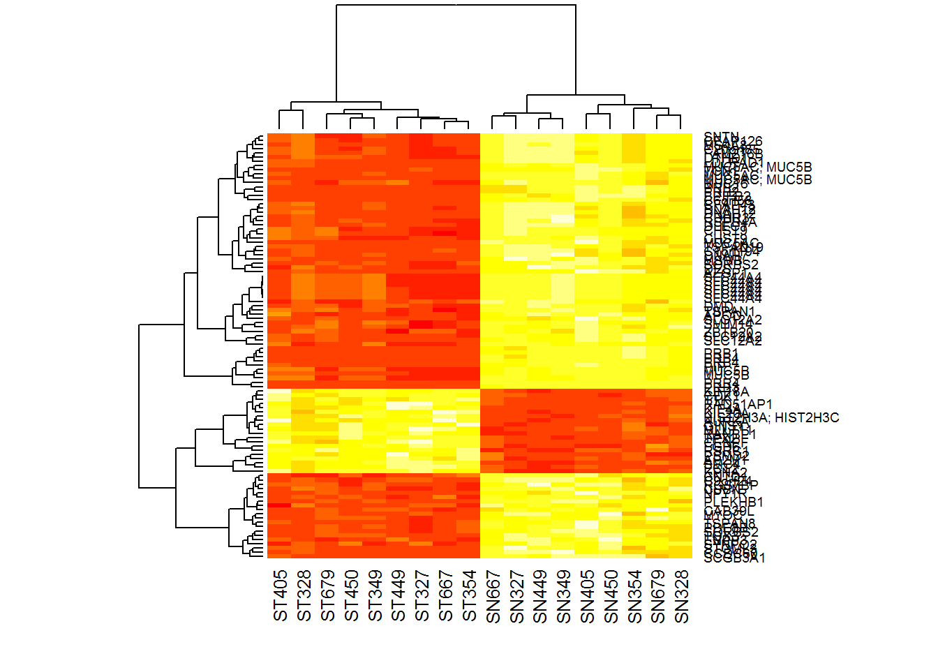
You can see here several issues. First, despite we visualize expression that is centered and scaled for each gene, we see strange clustering. ‘heatmap’ used the data itself, not standardized data to get clustering. Second, heatmaps are square, while we need here elongated to see the genes. Let’s use pheatmap.
library(pheatmap)
pheatmap(Xtop,scale="row",fontsize_row = 6)
4.1.3 DEA.limma - warp-up of the standard limma analysis
The small library LibDEA was created to speed up analysis of array and sequencing results. Let’s use it for faster analysis.
## get library
source("http://sablab.net/scripts/LibDEA.r")

## and run the fucntion
Res = DEA.limma(X, groups, key0="SN", key1="ST")
##
## Limma,unpaired: 15381,9869,5593,3074 DEG (FDR<0.05, 1e-2, 1e-3, 1e-4)str(Res)## 'data.frame': 67528 obs. of 7 variables:
## $ id : chr "TC12003301.hg.1" "TC12001246.hg.1" "TC12002764.hg.1" "TC12003303.hg.1" ...
## $ logFC : num -11.6 -11.5 -10.6 -10.9 -10.4 ...
## $ AveExpr: num 13.1 12.3 11.6 11 11 ...
## $ t : num -86.9 -75 -43.9 -32.2 -31 ...
## $ P.Value: num 1.56e-25 2.34e-24 4.17e-20 1.16e-17 2.39e-17 ...
## $ FDR : num 1.06e-20 7.91e-20 9.39e-16 1.96e-13 3.05e-13 ...
## $ B : num 37.5 36.7 32.4 28.8 28.2 ...## take the same top 100
Top100 = Res[order(Res$FDR)[1:100],]
Xtop = X[rownames(Top100),]
rownames(Xtop) = Anno[rownames(Top100),"Gene.Symbol"]
pheatmap(Xtop,scale="row",fontsize_row = 6)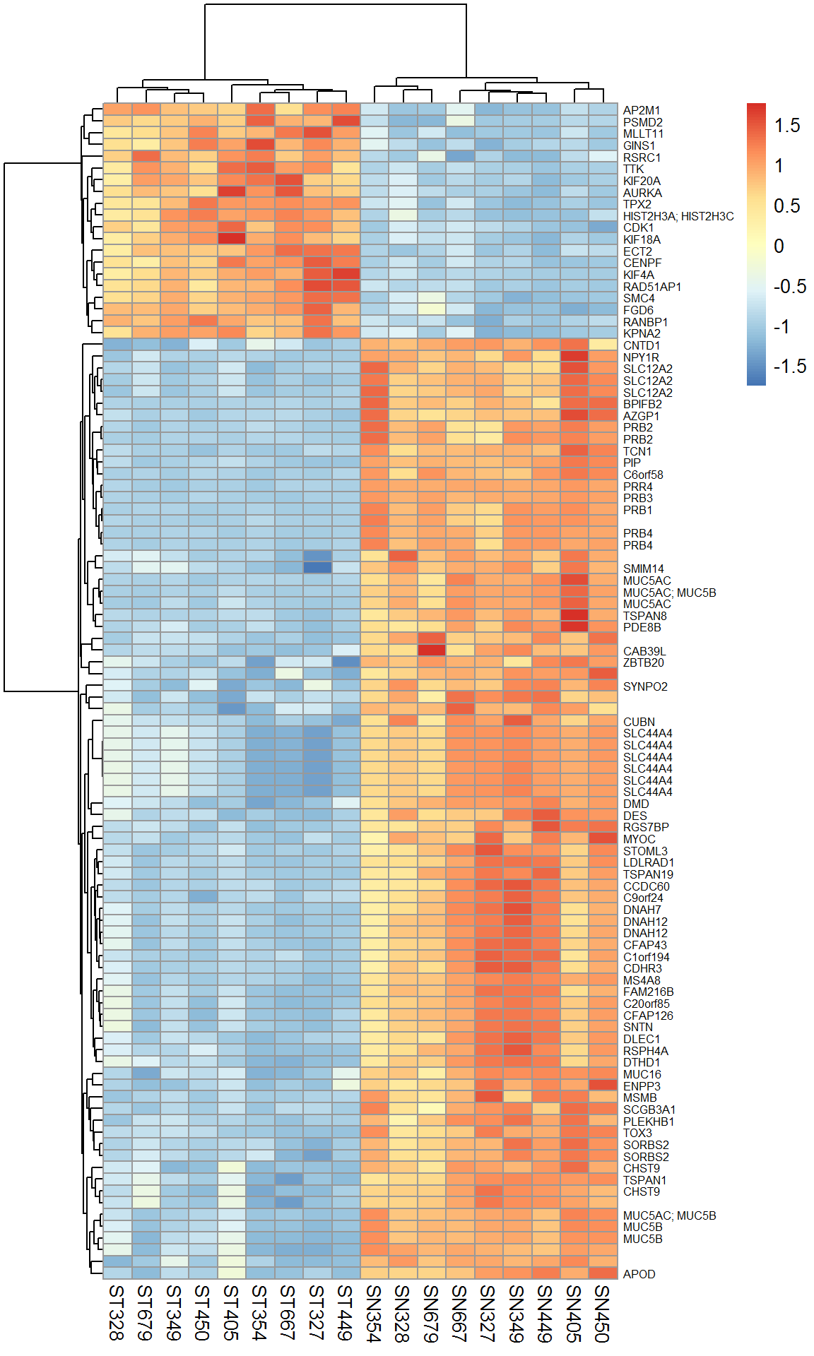
Let’s account for the patient effect and calculate expression for paired analysis. See effect for patient 450 and TNXB.
## get library
source("http://sablab.net/scripts/LibDEA.r")

## and run the fucntion
Res = DEA.limma(X, groups, pair = people, key0="SN", key1="ST")
##
## Limma,paired: 16002,9332,4111,1228 DEG (FDR<0.05, 1e-2, 1e-3, 1e-4)str(Res)## 'data.frame': 67528 obs. of 7 variables:
## $ id : chr "TC12003301.hg.1" "TC12001246.hg.1" "TC12002764.hg.1" "TC12003303.hg.1" ...
## $ logFC : num -11.6 -11.5 -10.6 -10.9 -10.4 ...
## $ AveExpr: num 13.1 12.3 11.6 11 11 ...
## $ t : num -84.3 -80.1 -51.8 -36.1 -36.3 ...
## $ P.Value: num 3.77e-16 6.39e-16 6.09e-14 2.61e-12 2.46e-12 ...
## $ FDR : num 2.16e-11 2.16e-11 1.37e-09 2.93e-08 2.93e-08 ...
## $ B : num 20.6 20.5 19.1 17.2 17.2 ...## take the same top 100
Top100 = Res[order(Res$FDR)[1:100],]
Xtop = X[rownames(Top100),]
rownames(Xtop) = Anno[rownames(Top100),"Gene.Symbol"]
pheatmap(Xtop,scale="row",fontsize_row = 6)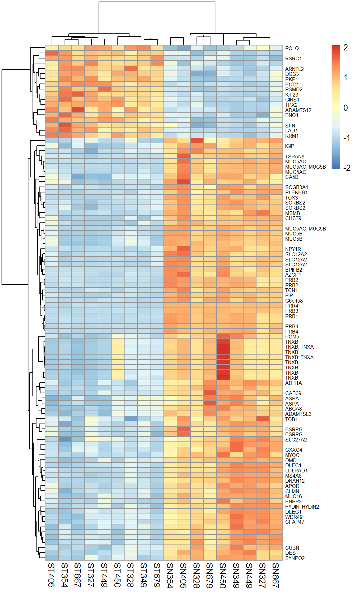
Finally, let’s save significant data, i.e. with FDR<0.01 to the disk.
str(Res)## 'data.frame': 67528 obs. of 7 variables:
## $ id : chr "TC12003301.hg.1" "TC12001246.hg.1" "TC12002764.hg.1" "TC12003303.hg.1" ...
## $ logFC : num -11.6 -11.5 -10.6 -10.9 -10.4 ...
## $ AveExpr: num 13.1 12.3 11.6 11 11 ...
## $ t : num -84.3 -80.1 -51.8 -36.1 -36.3 ...
## $ P.Value: num 3.77e-16 6.39e-16 6.09e-14 2.61e-12 2.46e-12 ...
## $ FDR : num 2.16e-11 2.16e-11 1.37e-09 2.93e-08 2.93e-08 ...
## $ B : num 20.6 20.5 19.1 17.2 17.2 ...Res$id = Anno[rownames(Res),"Gene.Symbol"]
write.table(Res[Res$FDR<0.01,], "DEA_HTA.txt",col.names=NA,sep="\t",quote=FALSE)
4.2. Analysis of RNA-seq data
For simplicity, let’s consider here how to run our custom warp-up function to analyse RNA-Seq data. If you are interested in using original Bioconductor functions - feel free to see in the code of LibDEA
Let’s consider the following libraries:
- DESeq2 is the one most often used (subjective), but it is also the slowest one (objective). It needs raw counts (negative binomial model of signal). It is developed by the group of Wolgang Huber (Heidelberg)
- edgeR . It needs raw counts (negative binomial model of signal). It is developed by the group of Gordon Smyth (Australia)
- limma . It can work with any form of expression (use
voomto transform from counts to log-expression). It is as well developed by the group of Gordon Smyth (Australia)
## load data
Data = read.table("http://edu.sablab.net/rt2018/data/counts.txt",header=T,sep="\t",row.names = 1)
str(Data)
## 'data.frame': 60411 obs. of 18 variables:
## $ SN327: int 11404 95 5058 4015 4137 266 77088 98 29717 1285 ...
## $ SN328: int 4652 112 4899 7001 6626 1161 41068 118 13984 1908 ...
## $ SN349: int 12880 107 5948 6573 4753 523 67236 169 25633 1952 ...
## $ SN354: int 5252 149 6508 5730 4728 813 56781 250 10469 1830 ...
## $ SN405: int 7752 169 4596 5858 2926 221 62818 159 13303 1326 ...
## $ SN449: int 12215 161 4009 4811 3754 620 70614 67 16995 1281 ...
## $ SN450: int 10898 86 5288 5010 3051 1012 107658 142 20073 1592 ...
## $ SN667: int 9793 370 4371 4905 3563 118 78049 98 27813 2248 ...
## $ SN679: int 7039 340 3560 4215 2478 949 62394 120 6482 1036 ...
## $ ST327: int 1768 32 3346 6450 8849 46 27302 125 165479 1653 ...
## $ ST328: int 3944 7 5062 6055 5424 1483 24056 185 47563 2947 ...
## $ ST349: int 4703 54 5837 7117 7773 644 22856 178 94699 2573 ...
## $ ST354: int 6323 247 8614 5027 8724 83 8912 79 8426 3487 ...
## $ ST405: int 1496 16 2546 4677 6252 120 27303 143 70070 1364 ...
## $ ST449: int 5547 33 4912 6942 9630 693 15821 217 87792 2248 ...
## $ ST450: int 6467 131 5055 4591 7006 1053 33937 101 104311 2242 ...
## $ ST667: int 2136 43 4608 3955 4599 180 14647 154 41703 1185 ...
## $ ST679: int 2778 123 1938 1945 2587 909 13117 179 6037 1818 ...## load annotation
Anno = read.table("http://edu.sablab.net/rt2018/data/counts_anno.txt",header=T,sep="\t",row.names = 1, as.is=TRUE)
Anno = Anno[rownames(Data),] ## force the same order
str(Anno)## 'data.frame': 60411 obs. of 8 variables:
## $ gene_name : chr "TSPAN6" "TNMD" "DPM1" "SCYL3" ...
## $ gene_biotype: chr "protein_coding" "protein_coding" "protein_coding" "protein_coding" ...
## $ seqname : chr "X" "X" "20" "1" ...
## $ start : int 99884983 99839799 49551773 169822913 169631245 27939633 196621008 143816984 53363765 41040684 ...
## $ stop : int 99894942 99854882 49574900 169863148 169823221 27961576 196716634 143832548 53481684 41067715 ...
## $ strand : chr "-" "+" "-" "-" ...
## $ length : int 2968 1610 1207 3844 6354 3524 8144 2453 8463 3811 ...
## $ gc : num 0.441 0.425 0.398 0.445 0.423 ...source("http://sablab.net/scripts/LibDEA.r")
groups = sub("[0-9]+","",colnames(Data))
## using DESeq2
Res1 = DEA.DESeq(Data,groups,key0="SN",key1="ST")## Loading required package: DESeq2## Loading required package: S4Vectors## Loading required package: stats4## Loading required package: BiocGenerics## Loading required package: parallel##
## Attaching package: 'BiocGenerics'## The following object is masked _by_ '.GlobalEnv':
##
## plotPCA## The following objects are masked from 'package:parallel':
##
## clusterApply, clusterApplyLB, clusterCall, clusterEvalQ,
## clusterExport, clusterMap, parApply, parCapply, parLapply,
## parLapplyLB, parRapply, parSapply, parSapplyLB## The following object is masked from 'package:limma':
##
## plotMA## The following objects are masked from 'package:stats':
##
## IQR, mad, sd, var, xtabs## The following objects are masked from 'package:base':
##
## anyDuplicated, append, as.data.frame, cbind, colMeans,
## colnames, colSums, do.call, duplicated, eval, evalq, Filter,
## Find, get, grep, grepl, intersect, is.unsorted, lapply,
## lengths, Map, mapply, match, mget, order, paste, pmax,
## pmax.int, pmin, pmin.int, Position, rank, rbind, Reduce,
## rowMeans, rownames, rowSums, sapply, setdiff, sort, table,
## tapply, union, unique, unsplit, which, which.max, which.min##
## Attaching package: 'S4Vectors'## The following object is masked from 'package:base':
##
## expand.grid## Loading required package: IRanges## Loading required package: GenomicRanges## Loading required package: GenomeInfoDb## Loading required package: SummarizedExperiment## Loading required package: Biobase## Welcome to Bioconductor
##
## Vignettes contain introductory material; view with
## 'browseVignettes()'. To cite Bioconductor, see
## 'citation("Biobase")', and for packages 'citation("pkgname")'.## Loading required package: DelayedArray## Loading required package: matrixStats##
## Attaching package: 'matrixStats'## The following objects are masked from 'package:Biobase':
##
## anyMissing, rowMedians##
## Attaching package: 'DelayedArray'## The following objects are masked from 'package:matrixStats':
##
## colMaxs, colMins, colRanges, rowMaxs, rowMins, rowRanges## The following object is masked from 'package:base':
##
## apply## estimating size factors## estimating dispersions## gene-wise dispersion estimates## mean-dispersion relationship## final dispersion estimates## fitting model and testing## -- replacing outliers and refitting for 1814 genes
## -- DESeq argument 'minReplicatesForReplace' = 7
## -- original counts are preserved in counts(dds)## estimating dispersions## fitting model and testing##
## DESeq,unpaired: 11918 DEG (FDR<0.05), 8913 DEG (FDR<0.01)## using edgeR
Res2 = DEA.edgeR(Data,groups,key0="SN",key1="ST")## Loading required package: edgeR##
## edgeR,unpaired: 8566 DEG (FDR<0.05), 5990 DEG (FDR<0.01)## using edgeR
Res3 = DEA.limma(Data,groups,key0="SN",key1="ST",counted=TRUE)##
## Limma,unpaired: 9038,6004,3329,1767 DEG (FDR<0.05, 1e-2, 1e-3, 1e-4)## Venn diagram
library(gplots)##
## Attaching package: 'gplots'## The following object is masked from 'package:IRanges':
##
## space## The following object is masked from 'package:S4Vectors':
##
## space## The following object is masked from 'package:stats':
##
## lowessid1 = Res1[Res1$FDR<0.01 & abs(Res1$logFC)>1,"id"]
id2 = Res2[Res2$FDR<0.01 & abs(Res2$logFC)>1,"id"]
id3 = Res3[Res3$FDR<0.01 & abs(Res3$logFC)>1,"id"]
venn(list(DESeq = id1, edgeR=id2, limma = id3))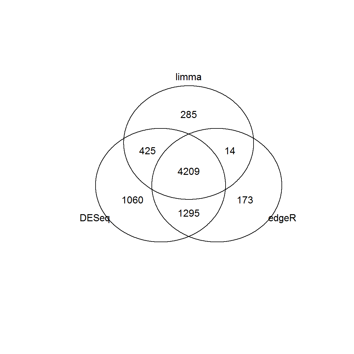
## alternative Venn
# source("http://sablab.net/scripts/Venn.r")
# v = Venn(list(DESeq = id1, edgeR=id2, limma = id3))
- Analyze dataset LUSC60 using one of the methods (DESeq2, edgeR or limma) and compare the gene lists to those found in LIH dataset counts. Hint: you will need to translate genes from Ensembl to gene symbols
DEA.limma,DEA.DESeq,DEA.edgeRsub,venn
- Select the top 1000 of the significant genes either in LUSC60 or in counts, save gene names into a file and perform enrichment analysis using Enrichr tool of Icahn School of Medicine at Mount Sinai, NY, USA.
write
![]()