3.1. Check data distribution

rm(list=ls()) ## clean memory
## download the data (in case you have not downloaded it before)
setwd("D:/Data/R") # sets the current folder
download.file("http://edu.sablab.net/rt2018/data/LUSC60.RData", destfile="LUSC60.RData",mode = "wb")

Now let’s investigate the data: see the content and distributions (remember - right skewed data are hard to work with!)

load("LUSC60.RData") # load the data
ls()

## [1] "Anno"      "color"     "Data"      "ensg"      "LUSC"      "oncogenes"
## [7] "X"         "XAnno"

## what is inside?
str(LUSC)

## List of 5
##  $ nsamples : num 60
##  $ nfeatures: int 20531
##  $ anno     :'data.frame':   20531 obs. of  2 variables:
##   ..$ gene    : chr [1:20531] "?|100130426" "?|100133144" "?|100134869" "?|10357" ...
##   ..$ location: chr [1:20531] "chr9:79791679-79792806:+" "chr15:82647286-82708202:+;chr15:83023773-83084727:+" "chr15:82647286-82707815:+;chr15:83023773-83084340:+" "chr20:56064083-56063450:-" ...
##  $ meta     :'data.frame':   60 obs. of  5 variables:
##   ..$ id         : chr [1:60] "NT.1" "NT.2" "NT.3" "NT.4" ...
##   ..$ disease    : chr [1:60] "LUSC" "LUSC" "LUSC" "LUSC" ...
##   ..$ sample_type: chr [1:60] "NT" "NT" "NT" "NT" ...
##   ..$ platform   : chr [1:60] "ILLUMINA" "ILLUMINA" "ILLUMINA" "ILLUMINA" ...
##   ..$ aliquot_id : chr [1:60] "a7309f60-5fb7-4cd9-90e8-54d850b4b241" "cabf7b00-4cb0-4873-a632-a5ffc72df2c8" "ee465ac7-c842-4337-8bd4-58fb49fce9bb" "6178dbb9-01d2-4ba3-8315-f2add186879a" ...
##  $ counts   : num [1:20531, 1:60] 0 3 13 272 1516 ...
##   ..- attr(*, "dimnames")=List of 2
##   .. ..$ : chr [1:20531] "?|100130426" "?|100133144" "?|100134869" "?|10357" ...
##   .. ..$ : chr [1:60] "NT.1" "NT.2" "NT.3" "NT.4" ...

plot(density(LUSC$counts),lwd=2,col="blue",main="Data distribution")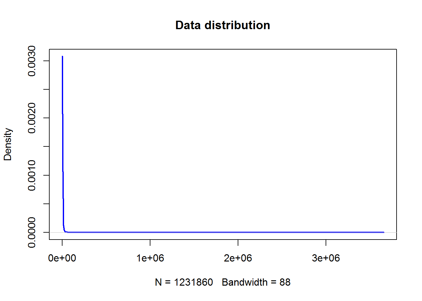

Higly right skewed! Need to do log2 transformation!

X = log2(1+LUSC$counts)
plot(density(X),lwd=2,col="blue",main="Data distribution (log scale)")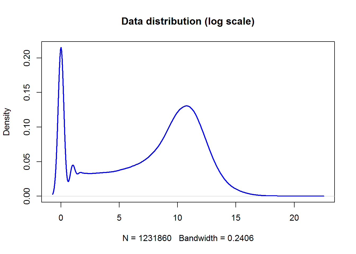

You can use my warp-up function plotDataPDF to see distribution of each samples

## load the script / function
source("http://sablab.net/scripts/plotDataPDF.r") 

## define colours
summary(as.factor(LUSC$meta$sample_type))

## NT TP 
## 20 40

color = c(TP = "#FF000055", NT = "#0000FF55")[LUSC$meta$sample_type]

## use warp-up function 
plotDataPDF(X,lwd=2,col=color,main="Distributions of gene expression in each sample")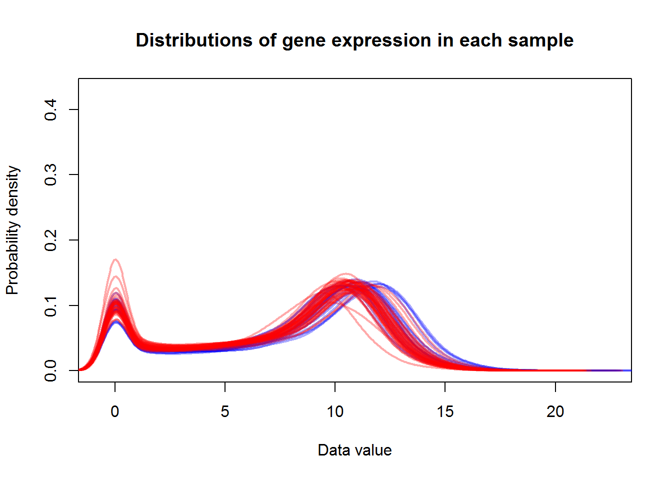

Conclusion: Data were highly right skewed. They were log2-transformed. Distributions are comparable.

3.2. PCA - Prinicipal Component Analysis

The standard function for PCA in R is prcomp. It considers rows as objects and columns as features. There are several limitations of prcomp:

It works only with matrix objects. => Please, transform your data.frame to matrix using as.matrix() function.
No NA values are allowed (please, impute or remove the features containing them)
No features of 0 variance are allowed (please, remove features that all are zeros)

There are more advanced PCA tools - Tony could comment :)

## perform PCA 
PC = prcomp(t(X))
str(PC)

## List of 5
##  $ sdev    : num [1:60] 119.2 72.6 46 39.3 36 ...
##  $ rotation: num [1:20531, 1:60] 1.65e-15 6.69e-05 -8.65e-04 7.38e-04 1.24e-03 ...
##   ..- attr(*, "dimnames")=List of 2
##   .. ..$ : chr [1:20531] "?|100130426" "?|100133144" "?|100134869" "?|10357" ...
##   .. ..$ : chr [1:60] "PC1" "PC2" "PC3" "PC4" ...
##  $ center  : Named num [1:20531] 0 4.85 4.8 8.6 11.1 ...
##   ..- attr(*, "names")= chr [1:20531] "?|100130426" "?|100133144" "?|100134869" "?|10357" ...
##  $ scale   : logi FALSE
##  $ x       : num [1:60, 1:60] -89.7 -128.5 -100.9 -159.4 -196.4 ...
##   ..- attr(*, "dimnames")=List of 2
##   .. ..$ : chr [1:60] "NT.1" "NT.2" "NT.3" "NT.4" ...
##   .. ..$ : chr [1:60] "PC1" "PC2" "PC3" "PC4" ...
##  - attr(*, "class")= chr "prcomp"

## plot PC1 and PC2 only
plot(PC$x[,1],PC$x[,2], col=color, pch=19)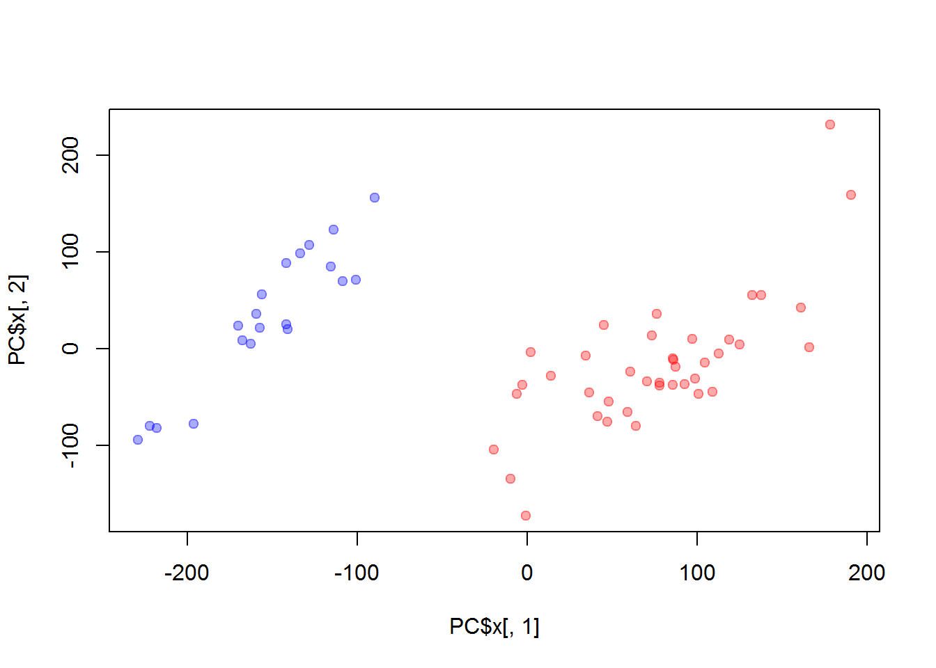

If you want, you can use a warp-up function for PCA plotPCA(). It takes care about some limitations (NAs, zero variance). No need to transpose data.

## load the script
source("http://sablab.net/scripts/plotPCA.r") 

## use our warp-up for PCA
plotPCA(X, col=color, pch=19, cex=2, cex.names=0.5)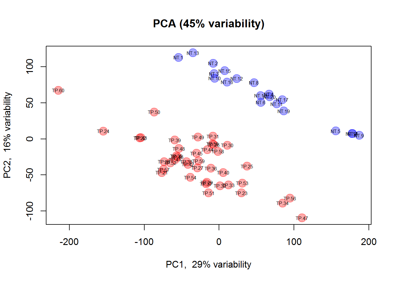

## add parameter scale=FALSE to get the same picture as before

You can also use 3D visualization:

## install package for 3D visualization
install.packages("rgl")
## load the package
library(rgl)
plot3d(PC$x[,1],PC$x[,2],PC$x[,3],
       size = 2,
       col  = color,
       type = "s",
       xlab = "PC1",
       ylab = "PC2",
       zlab = "PC3")

We considered samples as objects and genes as features. Now let’s do vice versa: genes as objects and samples as features.

## perform PCA - no transposition here  
PC2 = prcomp(X)
## plot PC1 and PC2 only
plot(PC2$x[,1],PC2$x[,2], col="#00880055", pch=19, cex = apply(X,1,mean)/10)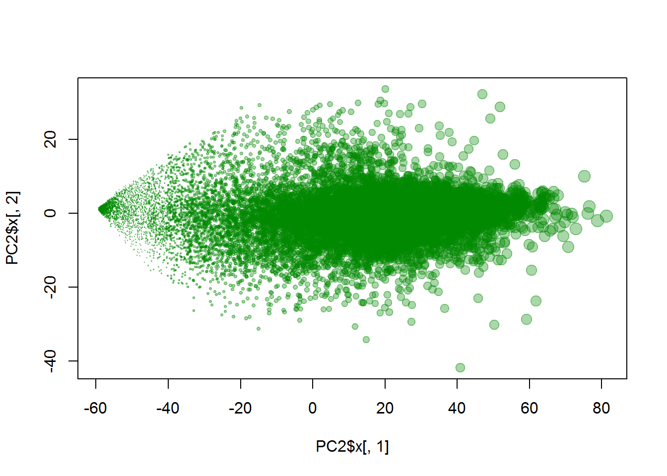

## for fun we used average expression to assign dot size :)

3.3 Correlations

Correlation can show linear agreement b/w samples (through the genes) or genes (through the samples). Let’s start with the first one. Please consider the range of correlation - this is usially the case for sample correlation in RNA-seq and one-colour arrays. Usually people use either Pearson (method="pearson") or Spearman (method="spearman").

RS = cor(X) ## try adding parameter method="spearman"
str(RS)

##  num [1:60, 1:60] 1 0.964 0.954 0.958 0.95 ...
##  - attr(*, "dimnames")=List of 2
##   ..$ : chr [1:60] "NT.1" "NT.2" "NT.3" "NT.4" ...
##   ..$ : chr [1:60] "NT.1" "NT.2" "NT.3" "NT.4" ...

## plot correlation matrix as a heatmap
library(pheatmap)
plot(density(RS),lwd=2,col="blue",main="Distribution of sample-sample correlation")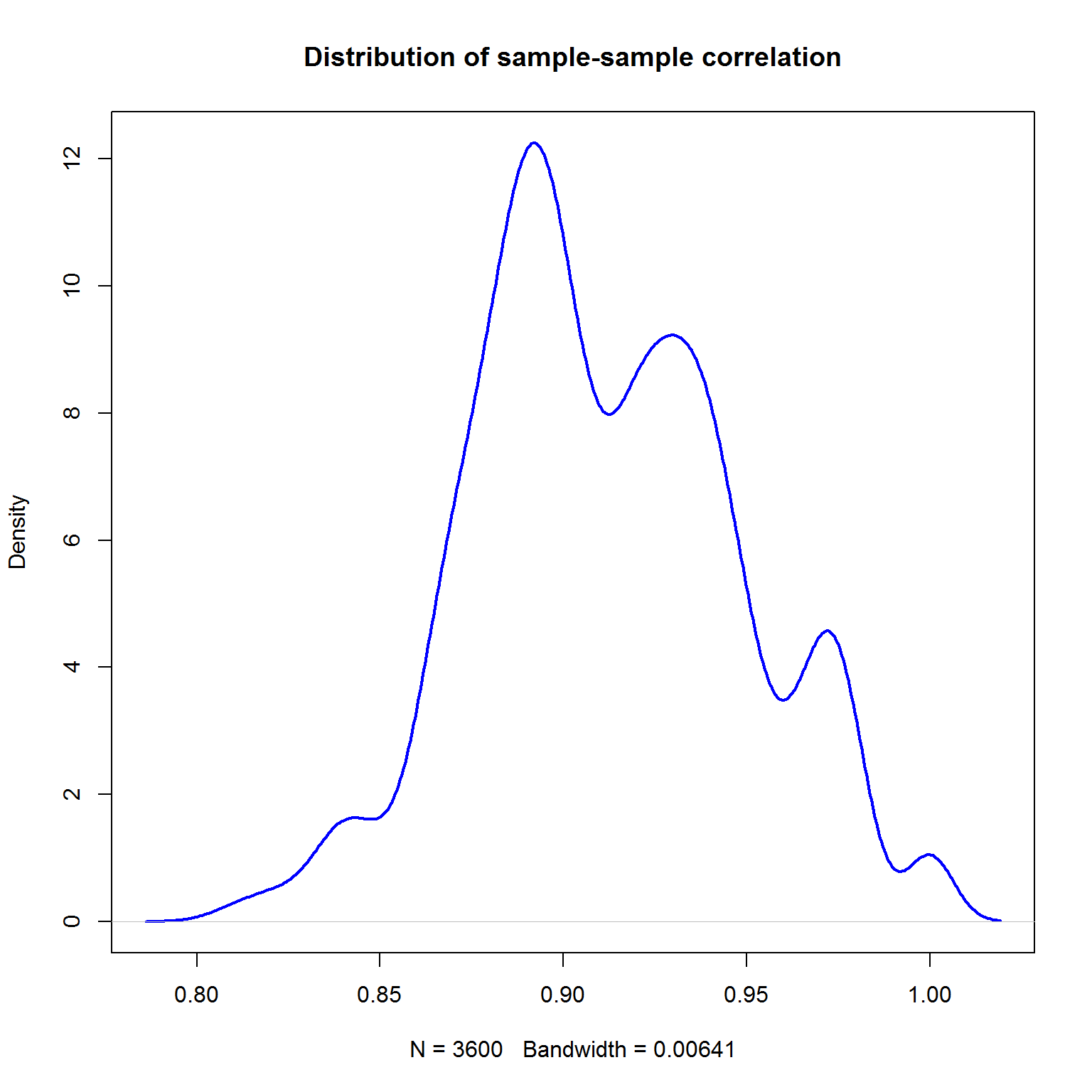

pheatmap(RS,main="Correlation b/w Samples")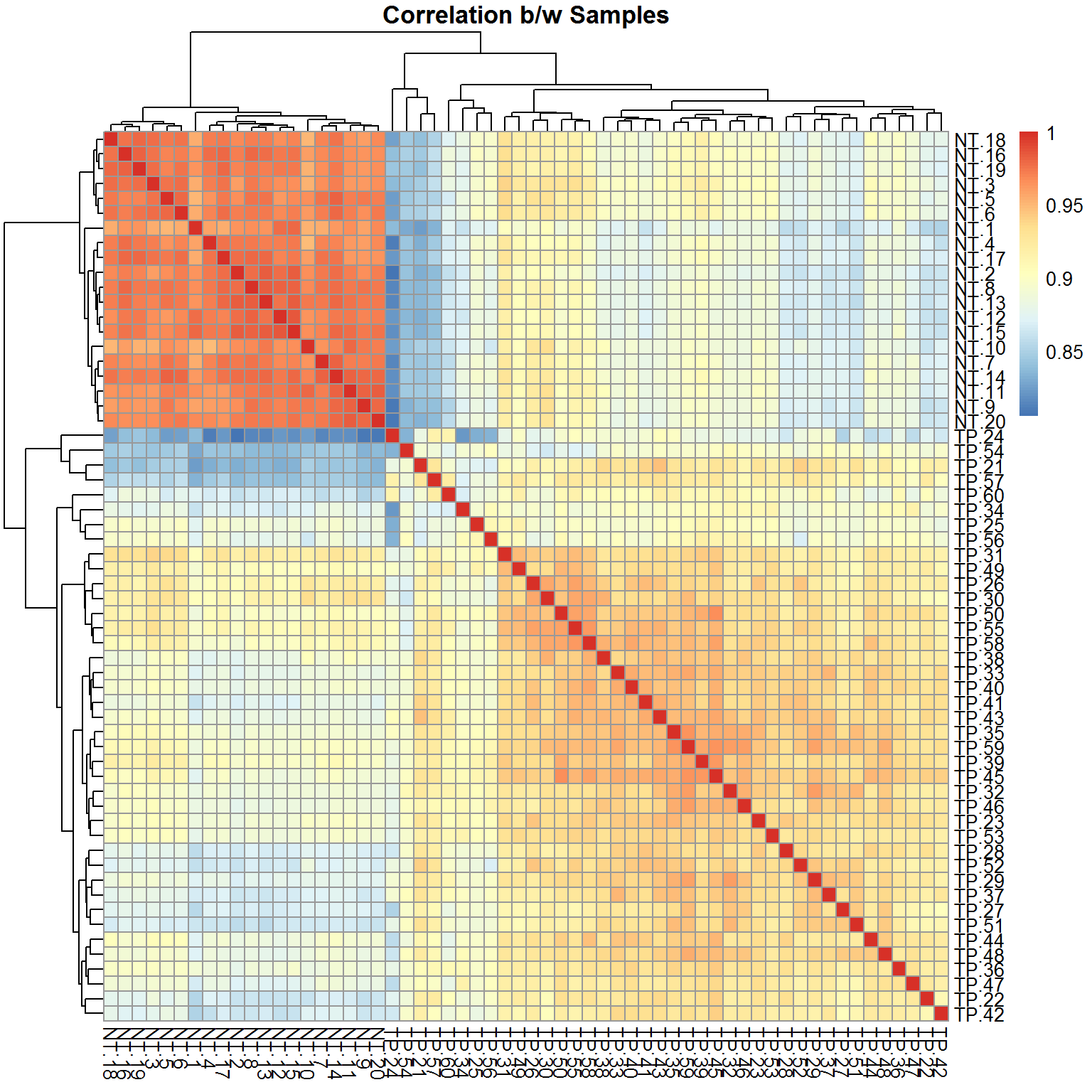

You could also correlate genes. Be prepared to get huge matrix! So, if you can, filter the genes first.

## filter the genes
ikeep = apply(X,1,max) > 7
ikeep = ikeep & apply(X,1,sd) > 1
sum(ikeep)

## [1] 9229

RG = cor(t(X[ikeep,]))
str(RG)

##  num [1:9229, 1:9229] 1 0.65 0.664 0.192 0.223 ...
##  - attr(*, "dimnames")=List of 2
##   ..$ : chr [1:9229] "?|100133144" "?|100134869" "?|155060" "?|340602" ...
##   ..$ : chr [1:9229] "?|100133144" "?|100134869" "?|155060" "?|340602" ...

plot(density(RG),lwd=2,col="red",main="Distribution of gene-gene correlation")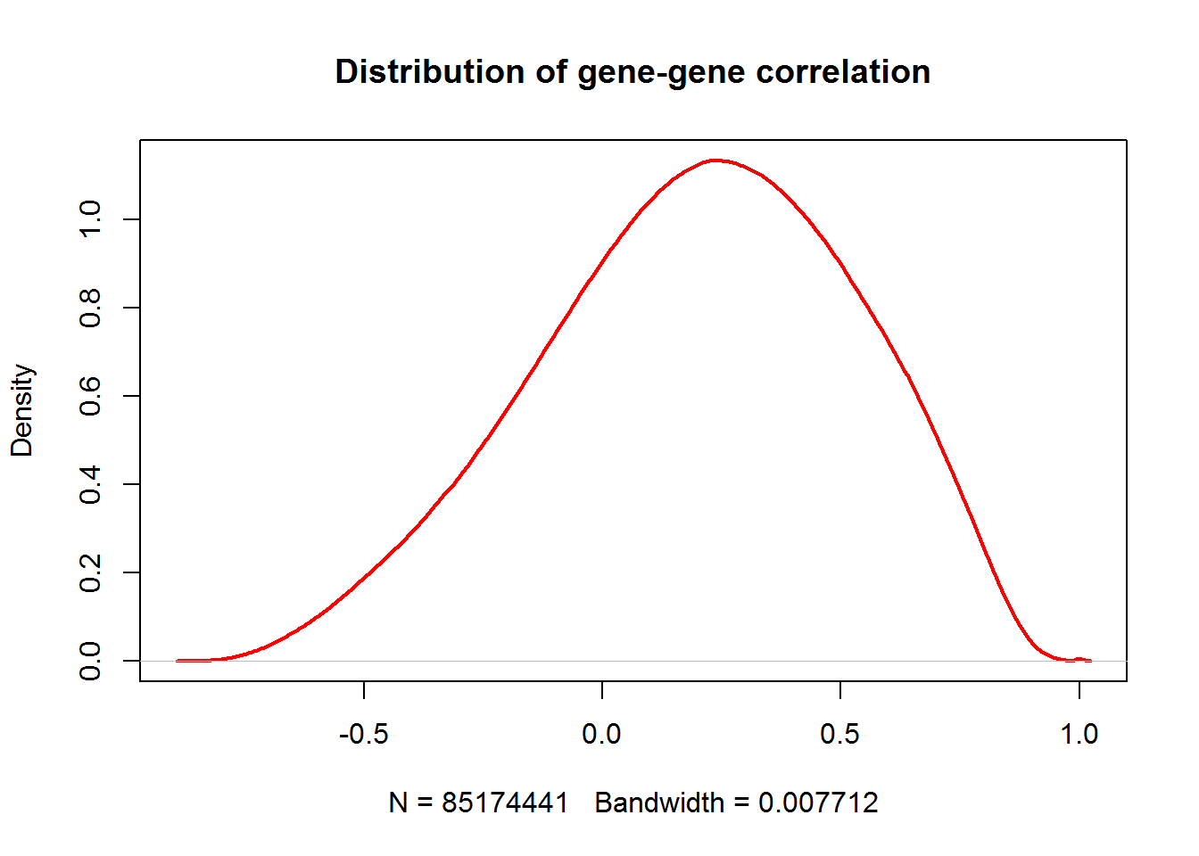

Excercises

Work with counts.txt data. Build distributions and perform necessary transformations. Perform PCA. Hint: Consider filtering out lowly expressed and invariable genes

density, log, apply, mean, max, sd, prcomp

Work with HTA.txt data. This dataset was obtained by HTA 2.0 arrays on the same samples as RNA-seq presented in counts.txt. Build distributions and transform data if needed. Perform PCA.

density,prcomp

Exploratory Analysis

Petr V. Nazarov, LIH

2018-03-05

3.1. Check data distribution

3.2. PCA - Prinicipal Component Analysis

3.3 Correlations

Excercises