- Differential Expression Analysis
Petr V. Nazarov, LIH
2019-11-21
5.1 Differentially Expression Analysis(DEA) - an approach
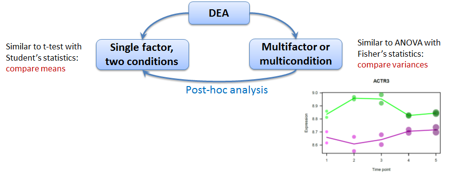
Approaches to detect differential genes
We will use limma (LInear Models for MicroArrays) that can do both F-test and (moderated) t-tests.
5.2 Library installation and data loading
## check whether limma is installed and instell if not
if (! "limma" %in% rownames(installed.packages()))
  install.packages("limma")

library(limma)
Now limma is installed. Let’s load the data
## load function readMaxQuant
source("http://sablab.net/scripts/readMaxQuant.r")

## load Data
Data = readMaxQuant(file = "http://edu.sablab.net/rp2019/data/proteinGroups.txt",
             key.data ="LFQ.intensity.",
             names.anno = c("Protein.names","Gene.names","Fasta.headers"),
             samples = "http://edu.sablab.net/rp2019/data/sampleAnnotation.txt",
             keep.na = FALSE,
             row.names=1,
             os.quantile=0.01)
## 5460 features were read.
## Reverse and contaminants are removed, resulting in 5306 features
## Remove 12 uninformative features
## [1] "Final data container:"
## List of 6
## $ nf : int 5294
## $ ns : int 19
## $ Anno:'data.frame': 5294 obs. of 3 variables:
## ..$ Protein.names: chr [1:5294] "Synapsin-3" "" "" "" ...
## ..$ Gene.names : chr [1:5294] "Syn3" "Abcf2" "Morc3" "Ddx17" ...
## ..$ Fasta.headers: chr [1:5294] "tr|A0A096MIT7|A0A096MIT7_RAT Synapsin-3 OS=Rattus norvegicus OX=10116 GN=Syn3 PE=1 SV=2;sp|O70441|SYN3_RAT Syna"| __truncated__ "tr|A0A096MIV5|A0A096MIV5_RAT ATP-binding cassette subfamily F member 2 OS=Rattus norvegicus OX=10116 GN=Abcf2 P"| __truncated__ "tr|D4A552|D4A552_RAT MORC family CW-type zinc finger 3 OS=Rattus norvegicus OX=10116 GN=Morc3 PE=1 SV=1;tr|A0A0"| __truncated__ "tr|E9PT29|E9PT29_RAT DEAD-box helicase 17 OS=Rattus norvegicus OX=10116 GN=Ddx17 PE=1 SV=3;tr|A0A096MIX2|A0A096"| __truncated__ ...
## $ Meta:'data.frame': 19 obs. of 2 variables:
## ..$ Time : chr [1:19] "day04" "day04" "day04" "day04" ...
## ..$ Replicate: chr [1:19] "rep1" "rep2" "rep3" "rep4" ...
## $ X0 : num [1:5294, 1:19] 2.15e+07 1.92e+07 1.37e+07 5.36e+08 1.20e+07 ...
## ..- attr(*, "dimnames")=List of 2
## .. ..$ : chr [1:5294] "A0A096MIT7;O70441" "A0A096MIV5;A2VD14;F1M8H5;A0A096MJ15" "D4A552;A0A096MIX0" "E9PT29;A0A096MIX2;A0A096MJW9" ...
## .. ..$ : chr [1:19] "BO2day4rep1" "BO2day4rep2" "BO2day4rep3" "BO2day4rep4" ...
## $ LX : num [1:5294, 1:19] 4.69 4.53 4.07 9.27 3.89 ...
## ..- attr(*, "dimnames")=List of 2
## .. ..$ : chr [1:5294] "A0A096MIT7;O70441" "A0A096MIV5;A2VD14;F1M8H5;A0A096MJ15" "D4A552;A0A096MIX0" "E9PT29;A0A096MIX2;A0A096MJW9" ...
## .. ..$ : chr [1:19] "BO2day4rep1" "BO2day4rep2" "BO2day4rep3" "BO2day4rep4" ...
5.3 Step-by-step
Limma works similar to ANOVA with somewhat improved post-hoc analysis and p-value calculation (empirical Bayes statistics). Let’s first see how to do simple analysis and then consider a warp-up function.
library(limma)
library(pheatmap)

## we will use Data$LX

## we should create factors
groups = factor(Data$Meta$Time)

## now create desigh matrix (a lot of FUN !)
design = model.matrix(~ -1 + groups)
colnames(design)=sub("groups","",colnames(design))
design
## day04 day10 day14 day21
## 1 1 0 0 0
## 2 1 0 0 0
## 3 1 0 0 0
## 4 1 0 0 0
## 5 1 0 0 0
## 6 0 1 0 0
## 7 0 1 0 0
## 8 0 1 0 0
## 9 0 1 0 0
## 10 0 1 0 0
## 11 0 0 1 0
## 12 0 0 1 0
## 13 0 0 1 0
## 14 0 0 1 0
## 15 0 0 1 0
## 16 0 0 0 1
## 17 0 0 0 1
## 18 0 0 0 1
## 19 0 0 0 1
## attr(,"assign")
## [1] 1 1 1 1
## attr(,"contrasts")
## attr(,"contrasts")$groups
## [1] "contr.treatment"## first fit: linear model
fit = lmFit(Data$LX,design=design)
## we will skip here F-test. See "LibDEA.r" why
## define contrast (post-hoc of ANOVA)
contrast.matrix = makeContrasts(day10-day04,day14-day04,day21-day04, levels=design)
contrast.matrix## Contrasts
## Levels day10 - day04 day14 - day04 day21 - day04
## day04 -1 -1 -1
## day10 1 0 0
## day14 0 1 0
## day21 0 0 1## second fit: contrasts
fit2 = contrasts.fit(fit,contrast.matrix)
EB = eBayes(fit2)
colnames(EB$coefficients)## [1] "day10 - day04" "day14 - day04" "day21 - day04"## get table of top 100 significant genes
Res10 = topTable(EB,1,number=100,adjust="BH")
Res14 = topTable(EB,2,number=100,adjust="BH")
Res21 = topTable(EB,3,number=100,adjust="BH")
str(Res10)## 'data.frame': 100 obs. of 6 variables:
## $ logFC : num 4.31 3.41 -2.52 2.76 3.96 ...
## $ AveExpr : num 3.978 2.975 0.664 2.389 12.263 ...
## $ t : num 44.4 36.6 -35.1 27.2 25.4 ...
## $ P.Value : num 8.38e-19 2.05e-17 4.07e-17 2.78e-15 8.47e-15 ...
## $ adj.P.Val: num 4.44e-15 5.43e-14 7.18e-14 3.68e-12 8.97e-12 ...
## $ B : num 32.1 29.5 28.9 25.1 24.1 ...## visualize
Top = Data$LX[rownames(Res10),]
rownames(Top) = substr(rownames(Top),1,20)
pheatmap(Top,fontsize_col=8,fontsize_row=4,scale="row",annotation_col = Data$Meta)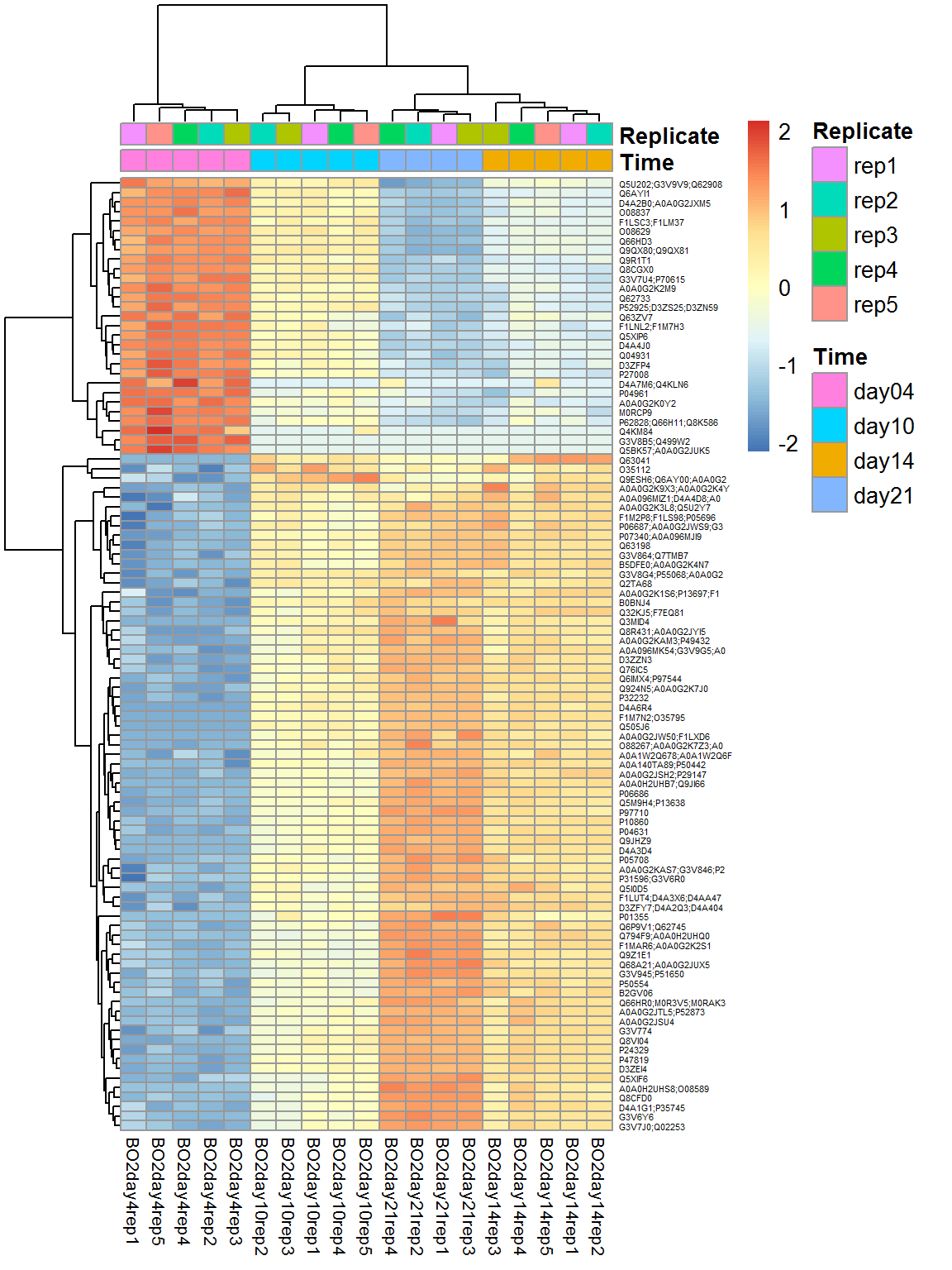
5.4 DEA.limma - warp-up of the standard limma analysis
The small library LibDEA was created to speed up analysis of array and sequencing results. Let’s use it for faster analysis. We can perform analysis using variances (F-test) and means (t-test).
## get library
source("http://sablab.net/scripts/LibDEA.r")

## and run the fucntion - this calculates FDR based on F-test
ResF = DEA.limma(Data$LX, group = Data$Meta$Time)
## [1] "day10-day04" "day14-day04" "day14-day10" "day21-day04" "day21-day10"
## [6] "day21-day14"
##
## Limma,unpaired: 3619,2971,2281,1732 DEG (FDR<0.05, 1e-2, 1e-3, 1e-4)str(ResF)## 'data.frame': 5294 obs. of 11 variables:
## $ id : chr "A0A096MIT7;O70441" "A0A096MIV5;A2VD14;F1M8H5;A0A096MJ15" "D4A552;A0A096MIX0" "E9PT29;A0A096MIX2;A0A096MJW9" ...
## $ day10.day04: num 0.156 -0.488 -0.236 -0.524 -1.706 ...
## $ day14.day04: num 0.117 -0.57 0.918 -1.026 -2.254 ...
## $ day14.day10: num -0.0392 -0.0824 1.1535 -0.5016 -0.5484 ...
## $ day21.day04: num -0.708 -0.696 0.832 -1.506 -3.029 ...
## $ day21.day10: num -0.865 -0.208 1.067 -0.983 -1.323 ...
## $ day21.day14: num -0.8254 -0.1253 -0.0864 -0.481 -0.7749 ...
## $ AveExpr : num 4.79 4.14 4.35 8.75 2.36 ...
## $ F : num 18.19 23.23 1.89 159.19 27.37 ...
## $ P.Value : num 1.64e-05 3.36e-06 1.71e-01 1.68e-12 1.10e-06 ...
## $ FDR : num 5.35e-05 1.31e-05 2.08e-01 9.86e-11 4.99e-06 ...## take the top 100
top_prots = rownames(ResF)[order(ResF$FDR)[1:100]]
Top = Data$LX[top_prots,]
pheatmap(Top,fontsize_col=8,fontsize_row=4,scale="row",annotation_col = Data$Meta)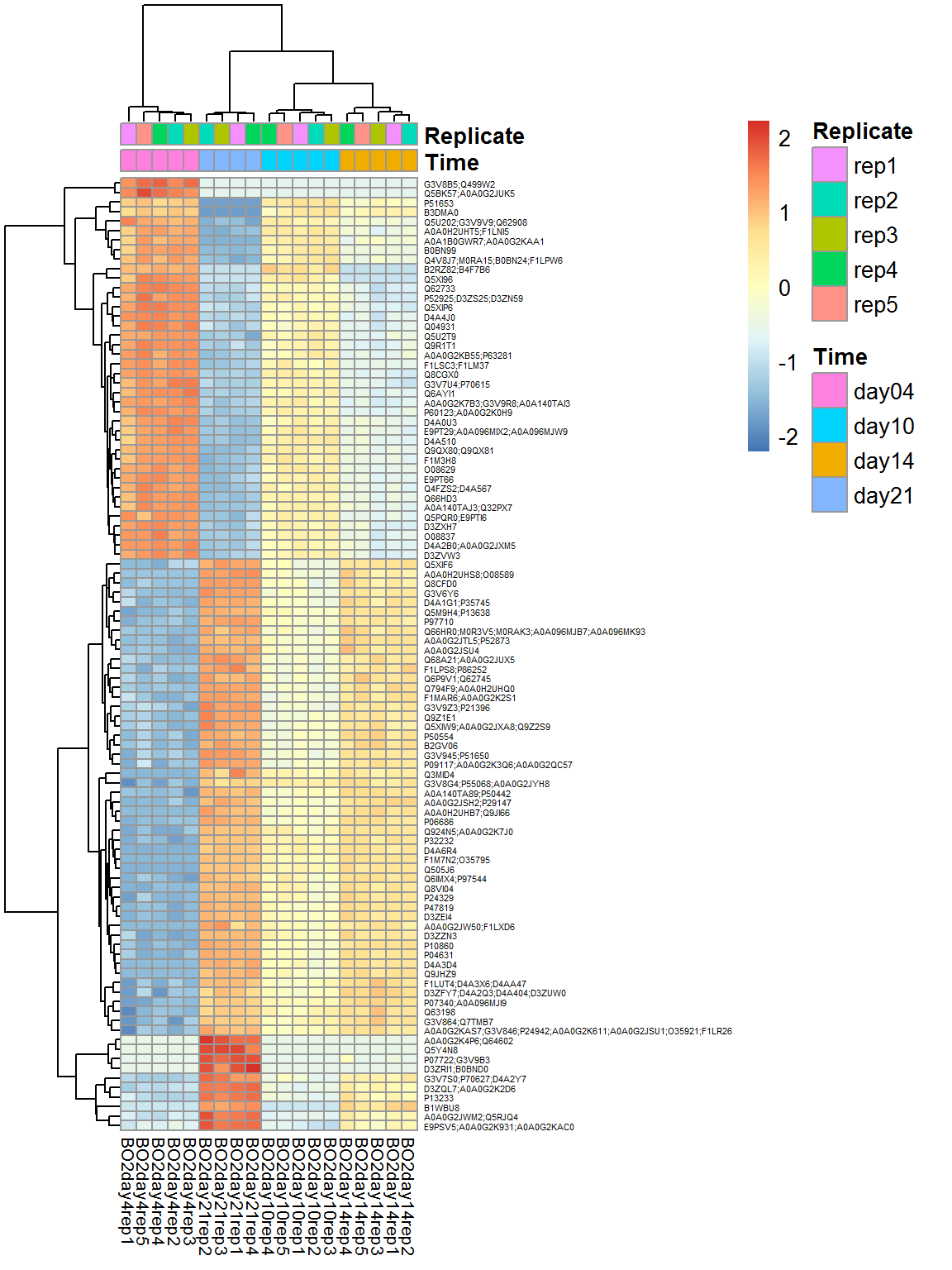
Now, perform analysis for each comparison
Res = DEA.limma(Data$LX, group = Data$Meta$Time, key0="day04", key1="day10")## Warning: Zero sample variances detected, have been offset away from zero##
## Limma,unpaired: 2006,1251,456,88 DEG (FDR<0.05, 1e-2, 1e-3, 1e-4)str(Res)## 'data.frame': 5294 obs. of 7 variables:
## $ id : chr "A0A096MIT7;O70441" "A0A096MIV5;A2VD14;F1M8H5;A0A096MJ15" "D4A552;A0A096MIX0" "E9PT29;A0A096MIX2;A0A096MJW9" ...
## $ logFC : num 0.156 -0.488 -0.236 -0.524 -1.706 ...
## $ AveExpr: num 4.94 4.33 3.87 9.21 3.18 ...
## $ t : num 1.459 -6.498 -0.315 -6.952 -5.628 ...
## $ P.Value: num 1.78e-01 9.71e-05 7.60e-01 5.72e-05 2.88e-04 ...
## $ FDR : num 0.277369 0.001064 0.837392 0.000773 0.002206 ...
## $ B : num -6.4623 1.2236 -7.4655 1.7899 0.0616 ...## take the same top 100
top_prots = rownames(Res)[order(Res$FDR)[1:100]]
Top = Data$LX[top_prots,]
pheatmap(Top,fontsize_col=8,fontsize_row=4,scale="row",annotation_col = Data$Meta)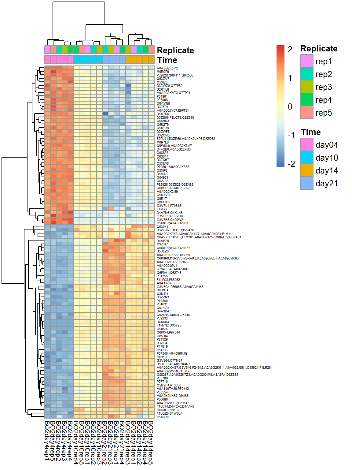
We can also visualize results using volcano plot
plot(Res$logFC, -log10(Res$FDR),col="#00000011",pch=19)
points(Res[top_prots,"logFC"], -log10(Res[top_prots,"FDR"]),col="#FF000055",pch=19)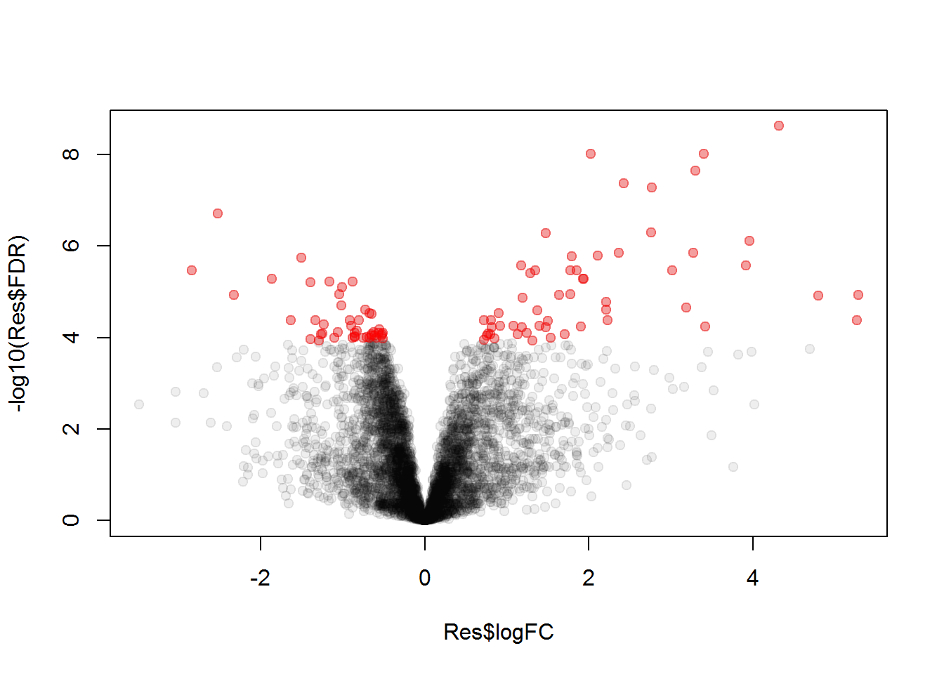
Finally, let’s save significant data, i.e. with FDR<0.01 to the disk.
write.table(Res[Res$FDR<0.01,], "DEA_example.txt",col.names=NA,sep="\t",quote=FALSE)
5.5. Venn diagram
Let us present the results using Venn diagram
## DEA
Res10 = DEA.limma(Data$LX,Data$Meta$Time,key0="day04",key1="day10")
## Warning: Zero sample variances detected, have been offset away from zero##
## Limma,unpaired: 2006,1251,456,88 DEG (FDR<0.05, 1e-2, 1e-3, 1e-4)Res14 = DEA.limma(Data$LX,Data$Meta$Time,key0="day04",key1="day14")## Warning: Zero sample variances detected, have been offset away from zero##
## Limma,unpaired: 3083,2351,1492,856 DEG (FDR<0.05, 1e-2, 1e-3, 1e-4)Res21 = DEA.limma(Data$LX,Data$Meta$Time,key0="day04",key1="day21")## Warning: Zero sample variances detected, have been offset away from zero##
## Limma,unpaired: 3617,3013,2181,1462 DEG (FDR<0.05, 1e-2, 1e-3, 1e-4)## Venn diagram
library(gplots)## Warning: package 'gplots' was built under R version 3.5.2##
## Attaching package: 'gplots'## The following object is masked from 'package:stats':
##
## lowessid10 = Res10[Res10$FDR<0.01 & abs(Res10$logFC)>1,"id"]
id14 = Res14[Res14$FDR<0.01 & abs(Res14$logFC)>1,"id"]
id21 = Res21[Res21$FDR<0.01 & abs(Res21$logFC)>1,"id"]
venn(list(day10 = id10, day14=id14, day21 = id21))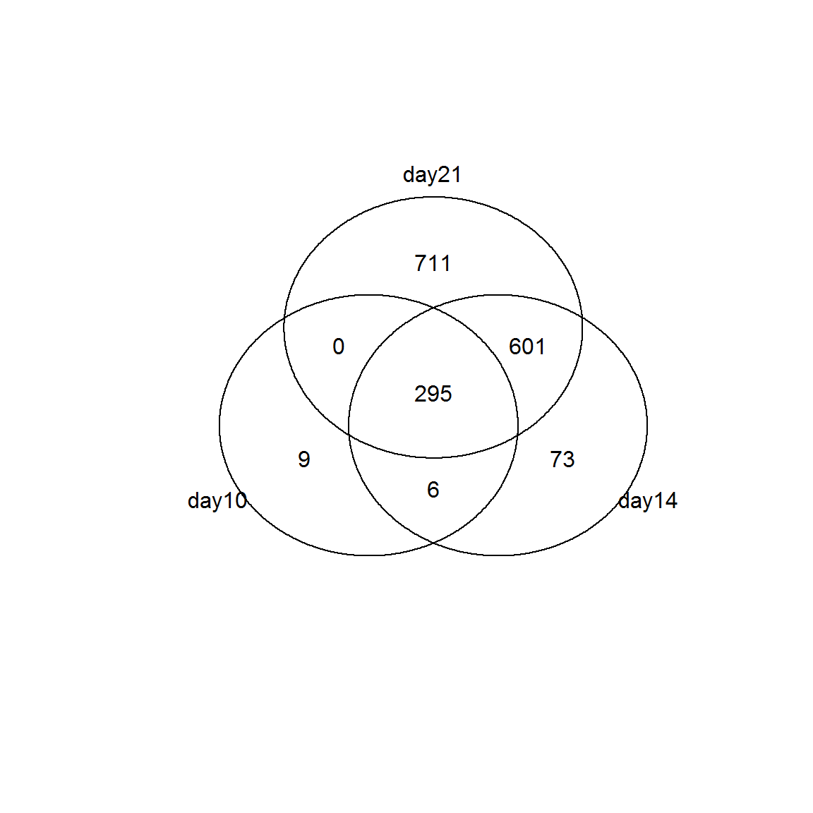
## alternative Venn
source("http://sablab.net/scripts/Venn.r")
v = Venn(list(day10 = id10, day14=id14, day21 = id21))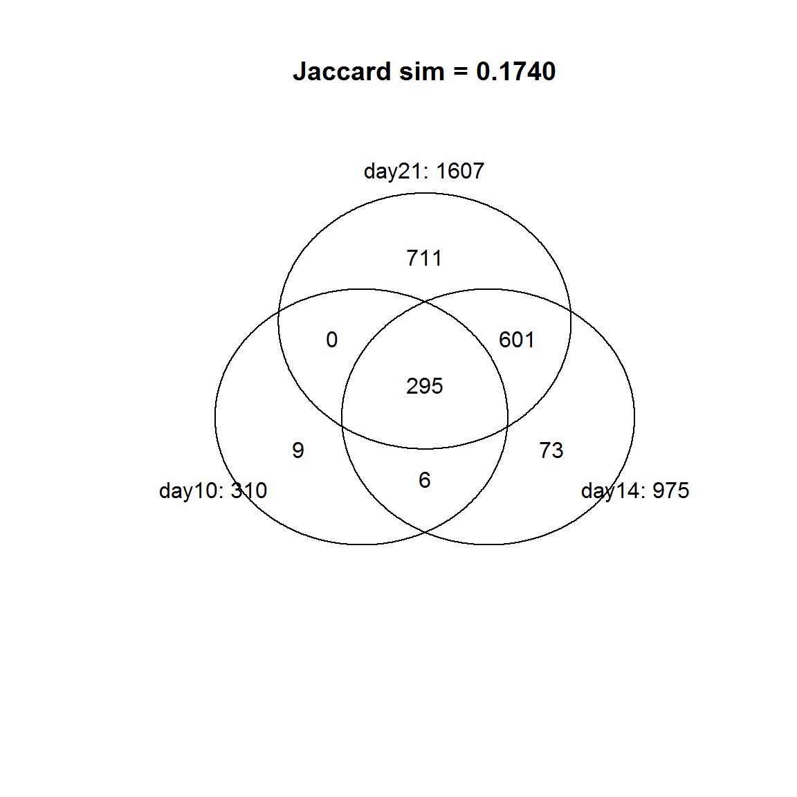
str(v)## 'venn' num [1:8, 1:4] 0 711 73 601 9 0 6 295 0 0 ...
## - attr(*, "dimnames")=List of 2
## ..$ : chr [1:8] "000" "001" "010" "011" ...
## ..$ : chr [1:4] "num" "day10: 310" "day14: 975" "day21: 1607"
## - attr(*, "intersections")=List of 6
## ..$ day10: 310 : chr [1:9] "A0A0G2JVG3;M0RD14" "D3ZNG0;D3ZBE9;F1M7T0;O88923" "D3ZN38" "D3ZNS8" ...
## ..$ day14: 975 : chr [1:73] "A0A096MKH4;D4ABY4" "A0A0G2JTD1" "A0A0G2JX93;Q66HB2" "A0A0G2JXG5" ...
## ..$ day21: 1607 : chr [1:711] "A0A096MJG7" "A0A096MJM1;Q32PX6;A0A096MK75" "A0A096MJY6" "A0A096MK73;P13668" ...
## ..$ day10: 310:day14: 975 : chr [1:6] "F1LWK7;A0A0G2K7Z4;A0A0G2JY49" "F1M8Y2;F1M9I6" "M0RC17" "P19686;Q5U330" ...
## ..$ day14: 975:day21: 1607 : chr [1:601] "E9PT29;A0A096MIX2;A0A096MJW9" "A0A096MJC5;B5DEN7;A0A096MJV2;D3Z8K0" "A0A096MJG1;Q5BKE0" "A0A0A0MXW1;P35738" ...
## ..$ day10: 310:day14: 975:day21: 1607: chr [1:295] "A1L1J2;F7EYN3;A0A096MIY3" "A0A096MIZ1;D4A4D8;A0A096MJ96" "A0A096MJE6;F1LQ63;Q05546" "A0A096MK54;G3V9G5;A0A096MKE8" ... ![]()