- Dimensionality reduction
Petr V. Nazarov, LIH
2019-11-21
Please, load the proteinGroups data as was shown earlier.
3.1. Overview of dimensionality reduction methods
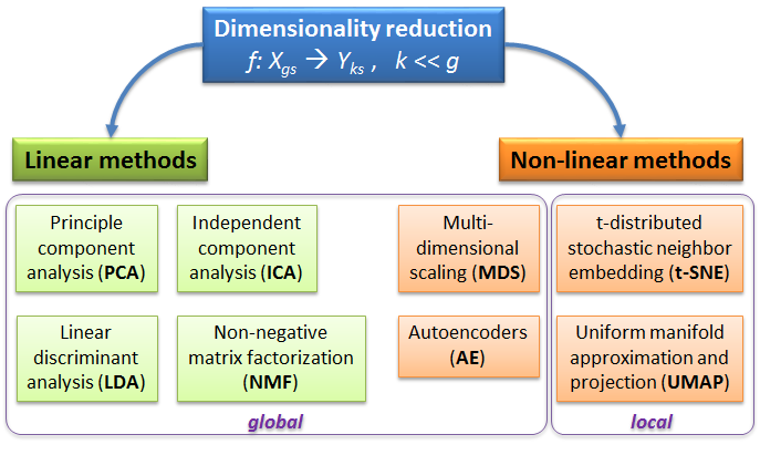
Some of the most used dimensionality reduction methods
PCA - rotation of the coordinate system in multidimensional space in the way to capture main variability in the data.
ICA - matrix factorization method that identifies statistically independent signals and their weights.
NMF - matrix factorization method that presents data as a matrix product of two non-negative matrices.
LDA - identify new coordinate system, maximizing difference between objects belonging to predefined groups.
MDS - method that tries to preserve distances between objects in the low-dimension space.
AE - artificial neural network with a “bottle-neck”.
t-SNE - an iterative approach, similar to MDS, but consideting only close objects. Thus, similar objects must be close in the new (reduced) space, while distant objects are not influecing the results.
UMAP - modern method, similar to t-SNE, but more stable and with preservation of some information about distant groups.
3.2. PCA
Simplest way to do PCA in R is to use default prcomp() function
PC = prcomp(t(Data$LX),scale=TRUE)
str(PC)
## List of 5
## $ sdev : num [1:19] 49.6 26.8 20.4 16.7 13.6 ...
## $ rotation: num [1:5294, 1:19] -0.01009 -0.0177 0.00687 -0.01992 -0.01849 ...
## ..- attr(*, "dimnames")=List of 2
## .. ..$ : chr [1:5294] "A0A096MIT7;O70441" "A0A096MIV5;A2VD14;F1M8H5;A0A096MJ15" "D4A552;A0A096MIX0" "E9PT29;A0A096MIX2;A0A096MJW9" ...
## .. ..$ : chr [1:19] "PC1" "PC2" "PC3" "PC4" ...
## $ center : Named num [1:5294] 4.79 4.14 4.35 8.75 2.36 ...
## ..- attr(*, "names")= chr [1:5294] "A0A096MIT7;O70441" "A0A096MIV5;A2VD14;F1M8H5;A0A096MJ15" "D4A552;A0A096MIX0" "E9PT29;A0A096MIX2;A0A096MJW9" ...
## $ scale : Named num [1:5294] 0.384 0.296 1.032 0.571 1.24 ...
## ..- attr(*, "names")= chr [1:5294] "A0A096MIT7;O70441" "A0A096MIV5;A2VD14;F1M8H5;A0A096MJ15" "D4A552;A0A096MIX0" "E9PT29;A0A096MIX2;A0A096MJW9" ...
## $ x : num [1:19, 1:19] -56.1 -70.4 -73.9 -68.8 -72.8 ...
## ..- attr(*, "dimnames")=List of 2
## .. ..$ : chr [1:19] "BO2day4rep1" "BO2day4rep2" "BO2day4rep3" "BO2day4rep4" ...
## .. ..$ : chr [1:19] "PC1" "PC2" "PC3" "PC4" ...
## - attr(*, "class")= chr "prcomp"plot(PC$x[,"PC1"],PC$x[,"PC2"],col=color,pch=19)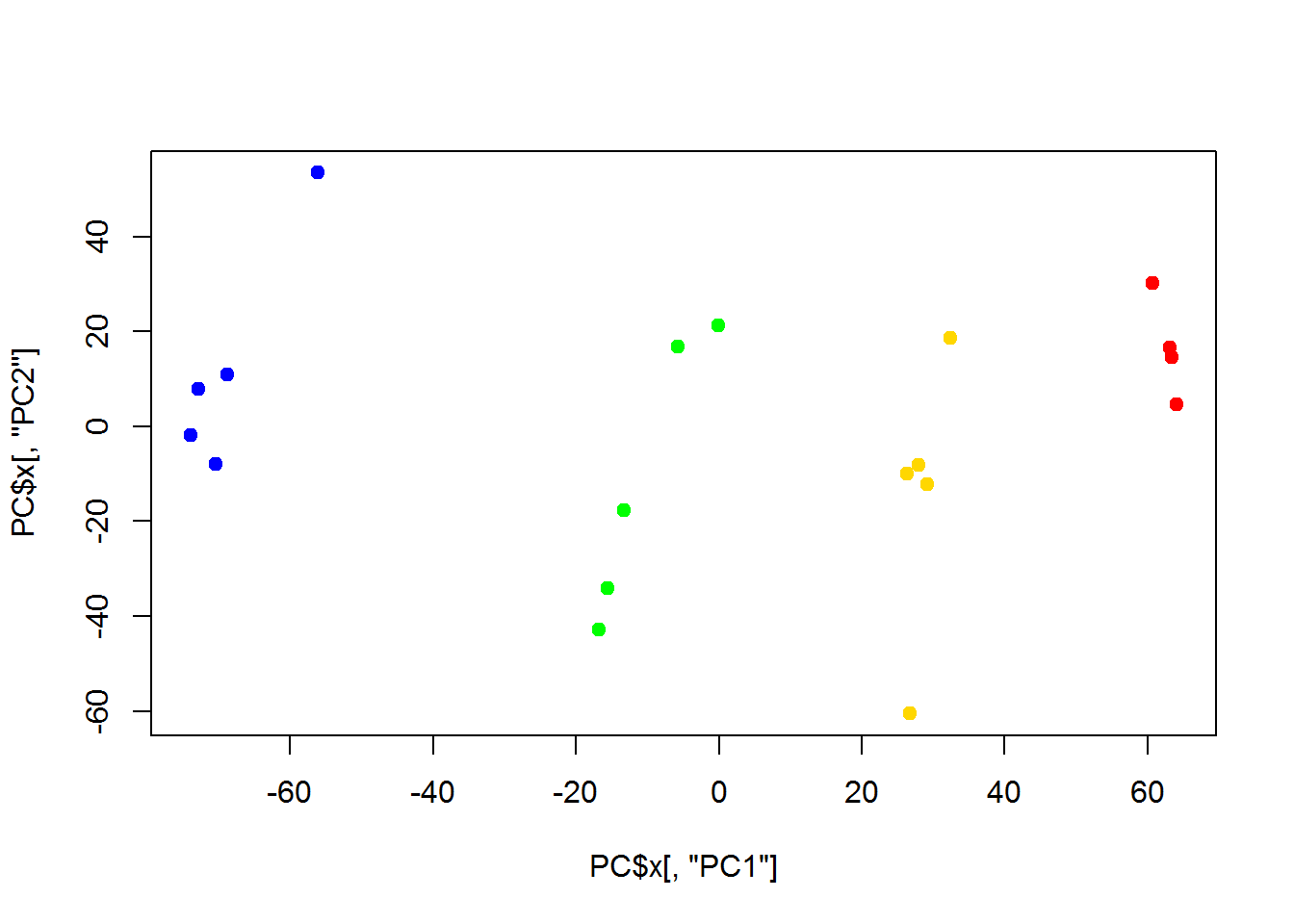
Alternatively you could use my warp-up function plotPCA()
source("http://sablab.net/scripts/plotPCA.r")
plotPCA(Data$LX,col=color)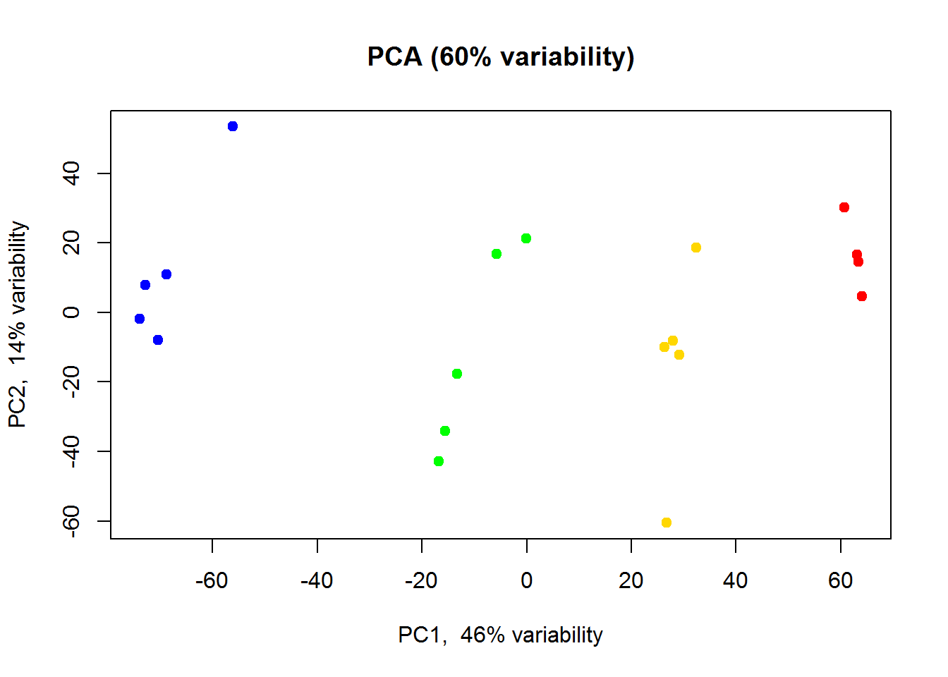
We can also use PCA to see similarity between features. Let’s also highlight marker genes.
markers = scan("http://edu.sablab.net/rp2019/data/markers.txt",what = "",sep="\n")
imarker = which(Data$Anno$Gene.names %in% markers)
color2 = rep("#0088FF33",Data$nf)
color2[imarker] = "#FF0000"
size = 0.5 + apply(Data$LX,1,mean)/6

## Log intensities
plotPCA(t(Data$LX),col=color2, cex=size)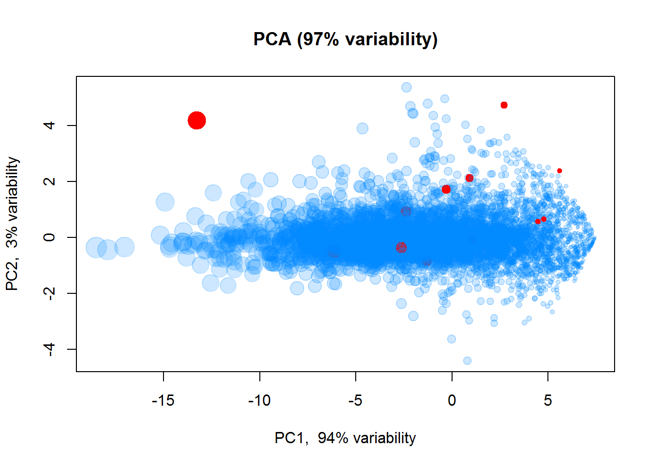
## Scaled log intensities
Z = Data$LX
Z[,] = t(scale(t(Z)))
plotPCA(t(Z),col=color2, cex=size)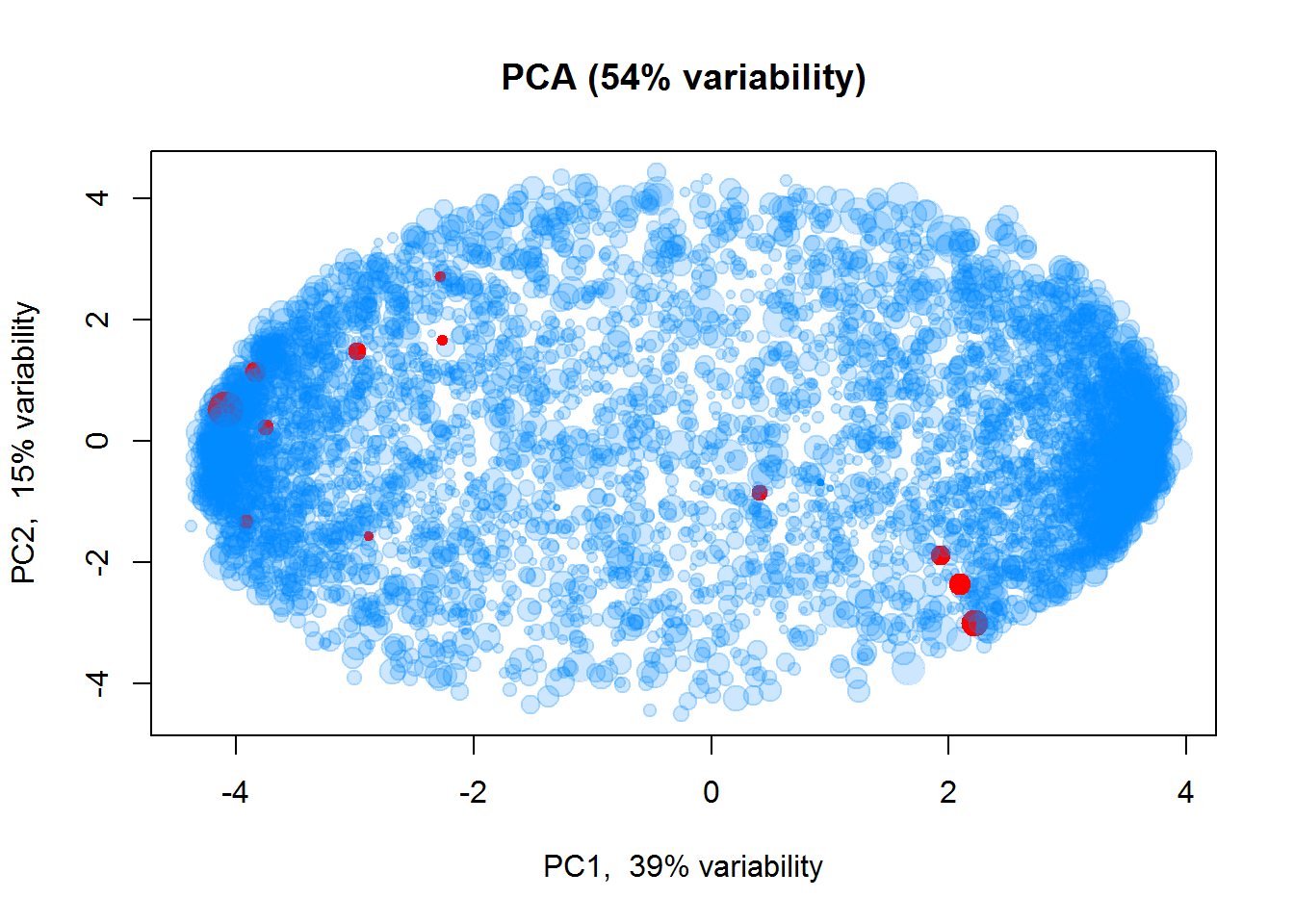
3.3. MDS
Classical MDS can be performed using cmdscale() function
## euclidean distances
d = dist(t(Data$LX))
## fit distances in 2D space to distances in multidimensional space
MDS = cmdscale(d,k=2)
str(MDS)
## num [1:19, 1:2] -40.9 -52.3 -52.5 -49.4 -52.9 ...
## - attr(*, "dimnames")=List of 2
## ..$ : chr [1:19] "BO2day4rep1" "BO2day4rep2" "BO2day4rep3" "BO2day4rep4" ...
## ..$ : NULLplot(MDS[,1],MDS[,2],col=color,pch=19, main="MDS plot")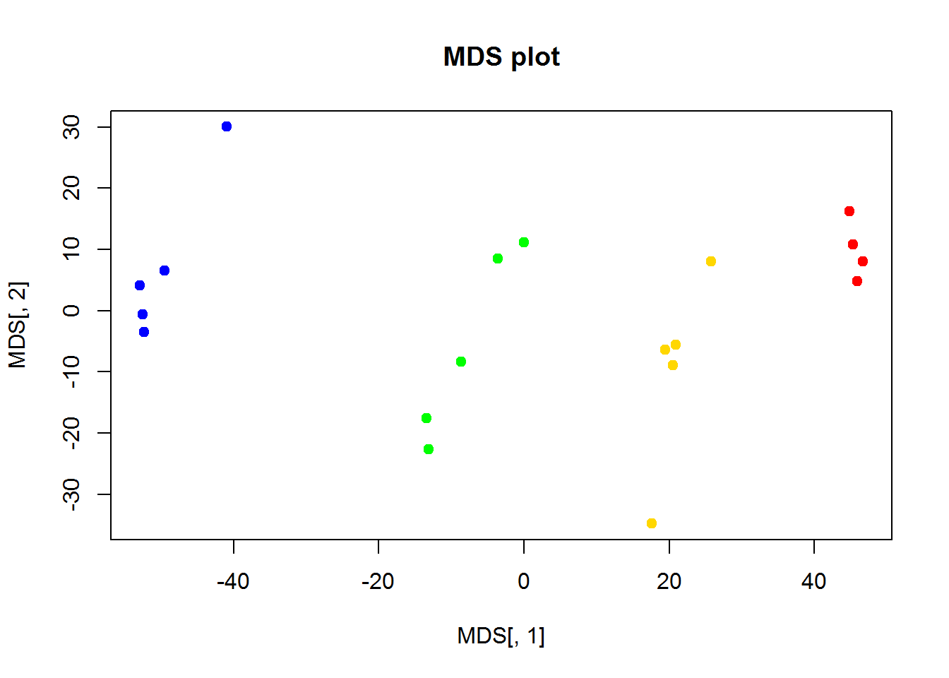
As you can see, it is very close to PCA results. But it requires much more computational power, when working with large number of objects. It may outperform PCA in a special case, when variance captured by 1st, 2nd and 3rd components is similar. Or when you need a special type of distance.
3.4. t-SNE
library(Rtsne)## Warning: package 'Rtsne' was built under R version 3.5.2TS1 = Rtsne(t(Data$LX),perplexity=3,max_iter=2000)$Y
plot(TS1[,1],TS1[,2],col=color,pch=19)
## plot features
TS2 = Rtsne(Data$LX,perplexity=20,max_iter=1000)$Y
plot(TS2[,1],TS2[,2],col=color2,pch=19,cex=size)
text(TS2[imarker,1],TS2[imarker,2],Data$Anno$Gene.names[imarker],font=2)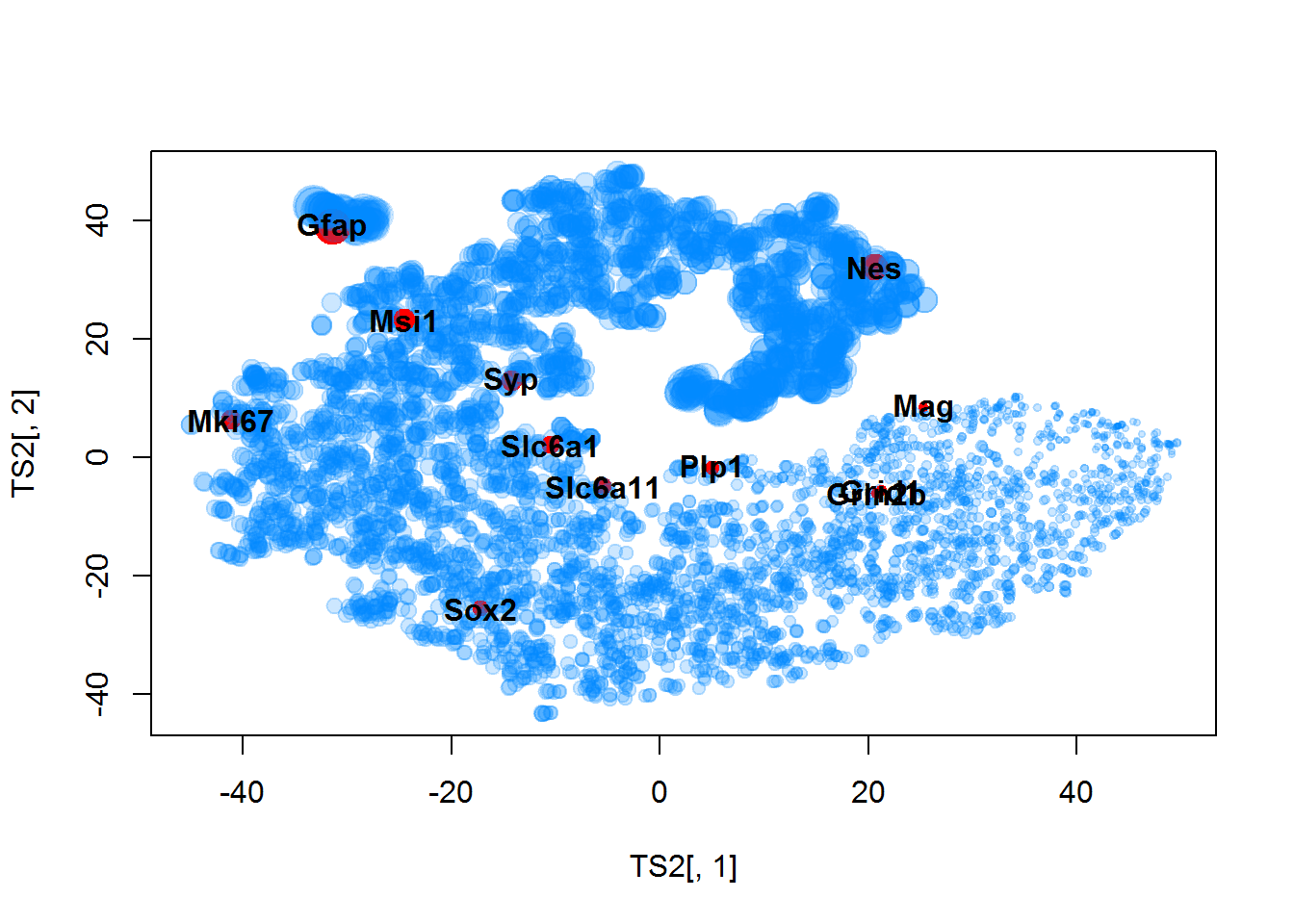
## same for scaled features
TS2 = Rtsne(Z,perplexity=100,max_iter=1000,check_duplicates = FALSE)$Y
plot(TS2[,1],TS2[,2],col=color2,pch=19,cex=size)
text(TS2[imarker,1],TS2[imarker,2],Data$Anno$Gene.names[imarker],font=2)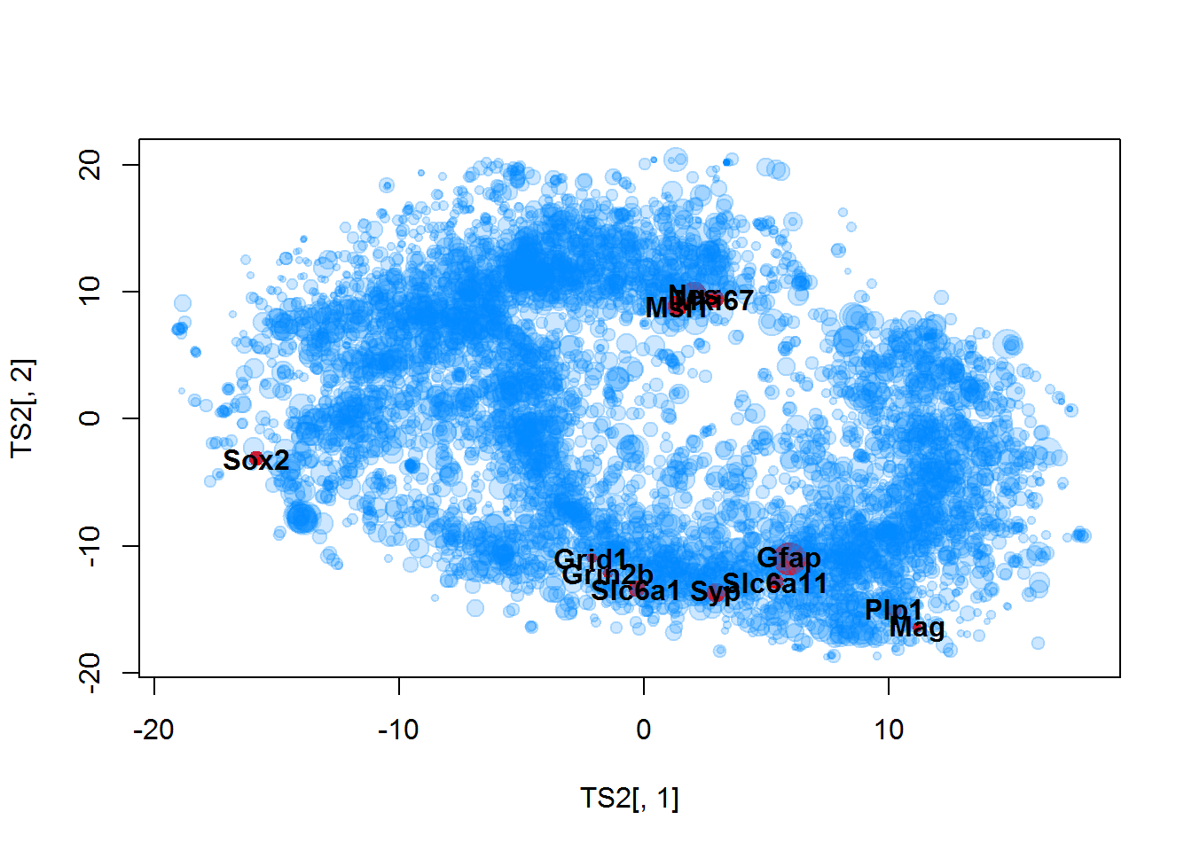
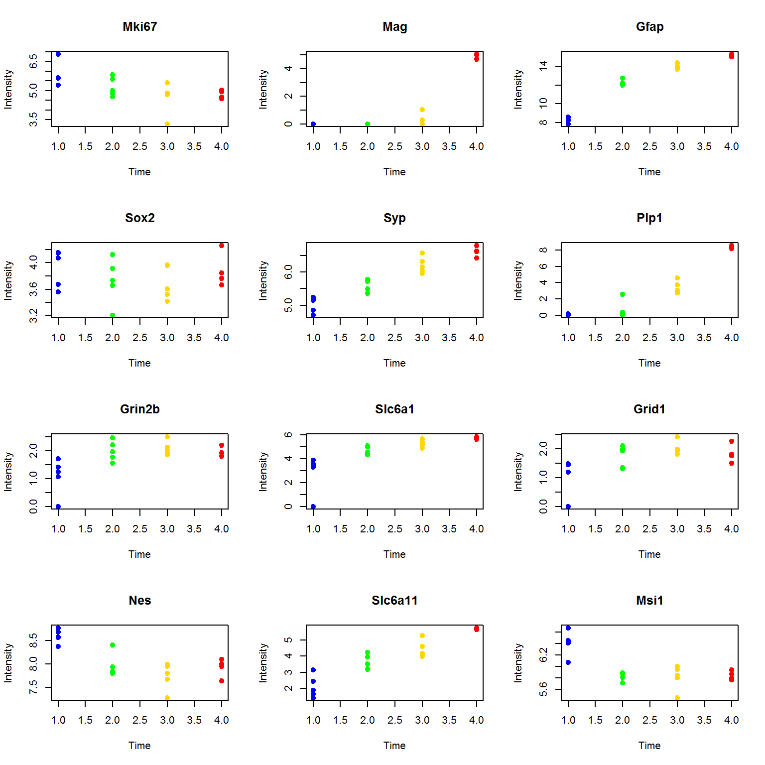
Let’s compare with profiles:
par(mfcol=c(4,3))
for (i in imarker){
  plot(as.integer(factor(Data$Meta$Time)),Data$LX[i,],pch=19,col=color,main=Data$Anno$Gene.names[i],xlab="Time",ylab="Intensity")
}
![]()