- Distributions
Petr V. Nazarov, LIH
2019-10-10
2.1. Boxplot
Let’s work again with proteinGroups file.
## load the script from Internet
source("http://sablab.net/scripts/readMaxQuant.r")

file = "D:/Data/RProteo2019/proteinGroups.txt"
## uncomment the following line to import from Internet
# file = "http://edu.sablab.net/rp2019/data/proteinGroups.txt"
Data = readMaxQuant(file,
             key.data = "LFQ.intensity.",
             names.anno = c("Protein.names","Gene.names","Fasta.headers"),
             samples = "http://edu.sablab.net/rp2019/data/sampleAnnotation.txt",
             keep.na = FALSE,
             row.names = 1,
             os.quantile = 0.01)
## 5460 features were read.
## Reverse and contaminants are removed, resulting in 5306 features
## Remove 12 uninformative features
## [1] "Final data container:"
## List of 6
## $ nf : int 5294
## $ ns : int 19
## $ Anno:'data.frame': 5294 obs. of 3 variables:
## ..$ Protein.names: chr [1:5294] "Synapsin-3" "" "" "" ...
## ..$ Gene.names : chr [1:5294] "Syn3" "Abcf2" "Morc3" "Ddx17" ...
## ..$ Fasta.headers: chr [1:5294] "tr|A0A096MIT7|A0A096MIT7_RAT Synapsin-3 OS=Rattus norvegicus OX=10116 GN=Syn3 PE=1 SV=2;sp|O70441|SYN3_RAT Syna"| __truncated__ "tr|A0A096MIV5|A0A096MIV5_RAT ATP-binding cassette subfamily F member 2 OS=Rattus norvegicus OX=10116 GN=Abcf2 P"| __truncated__ "tr|D4A552|D4A552_RAT MORC family CW-type zinc finger 3 OS=Rattus norvegicus OX=10116 GN=Morc3 PE=1 SV=1;tr|A0A0"| __truncated__ "tr|E9PT29|E9PT29_RAT DEAD-box helicase 17 OS=Rattus norvegicus OX=10116 GN=Ddx17 PE=1 SV=3;tr|A0A096MIX2|A0A096"| __truncated__ ...
## $ Meta:'data.frame': 19 obs. of 2 variables:
## ..$ Time : chr [1:19] "day04" "day04" "day04" "day04" ...
## ..$ Replicate: chr [1:19] "rep1" "rep2" "rep3" "rep4" ...
## $ X0 : num [1:5294, 1:19] 2.15e+07 1.92e+07 1.37e+07 5.36e+08 1.20e+07 ...
## ..- attr(*, "dimnames")=List of 2
## .. ..$ : chr [1:5294] "A0A096MIT7;O70441" "A0A096MIV5;A2VD14;F1M8H5;A0A096MJ15" "D4A552;A0A096MIX0" "E9PT29;A0A096MIX2;A0A096MJW9" ...
## .. ..$ : chr [1:19] "BO2day4rep1" "BO2day4rep2" "BO2day4rep3" "BO2day4rep4" ...
## $ LX : num [1:5294, 1:19] 4.69 4.53 4.07 9.27 3.89 ...
## ..- attr(*, "dimnames")=List of 2
## .. ..$ : chr [1:5294] "A0A096MIT7;O70441" "A0A096MIV5;A2VD14;F1M8H5;A0A096MJ15" "D4A552;A0A096MIX0" "E9PT29;A0A096MIX2;A0A096MJW9" ...
## .. ..$ : chr [1:19] "BO2day4rep1" "BO2day4rep2" "BO2day4rep3" "BO2day4rep4" ...Let us plot log-intensity as a boxplot.
boxplot()- command to plot boxplot
boxplot(Data$LX)Hmm… not too nice! Let’s improve
col- color of the barslas- axis text direction (2 for perpendicular)cex.names,cex.axis- size of the names on the catecorical axis and numerical axismain- title of the figure. Alterntivelytitle()can be called to add names after.xlab,ylab- names of axes
color = c(day04="blue",day10="green",day14="gold",day21="red")[Data$Meta$Time]

boxplot(Data$LX,
        las=2,
        cex.axis=0.7,
        pch=19,
        col=color,
        ylab="log intensity",
        main="Intensities in the samples")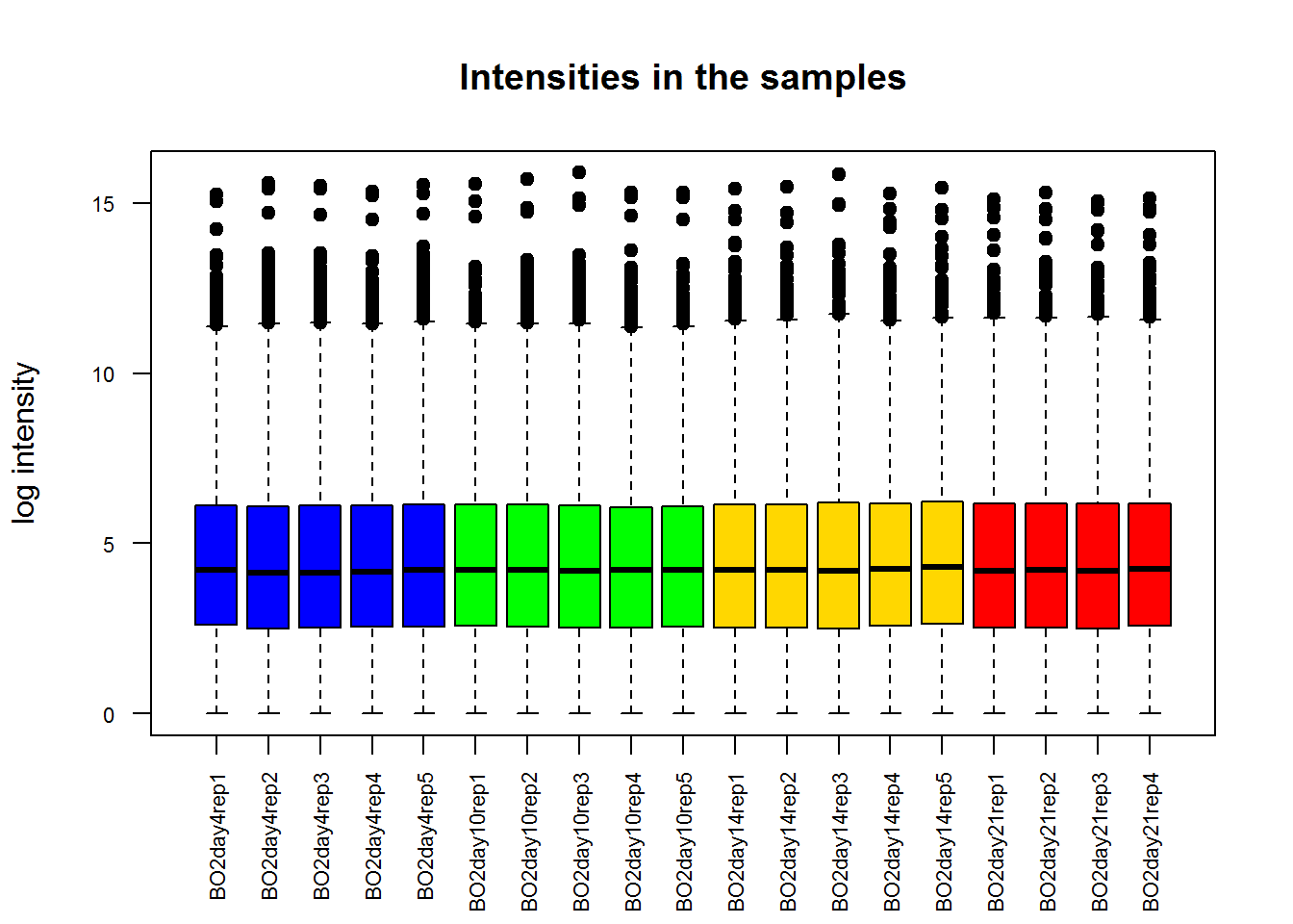
2.2. Density plots
Density plots can show you the distibution of the data. Let’s first see original intensities
plot(density(..))
plot(density(Data$X0),main="Original intensities",lwd=2,col="blue")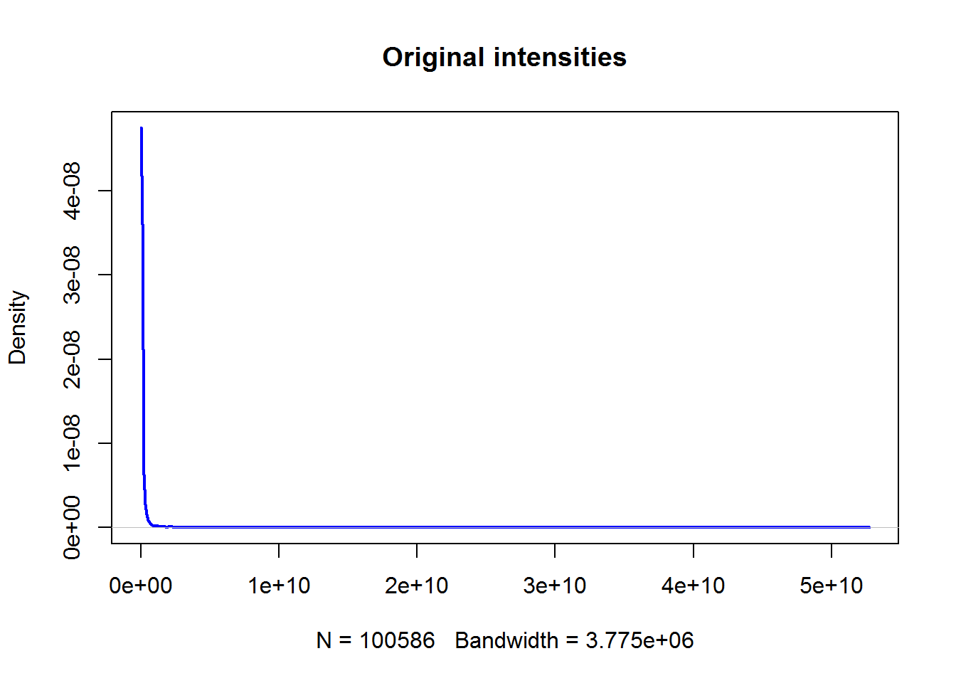
Not too interesting… And now log-transformed data:
plot(density(Data$LX),main="Log-intensities",lwd=2,col="blue")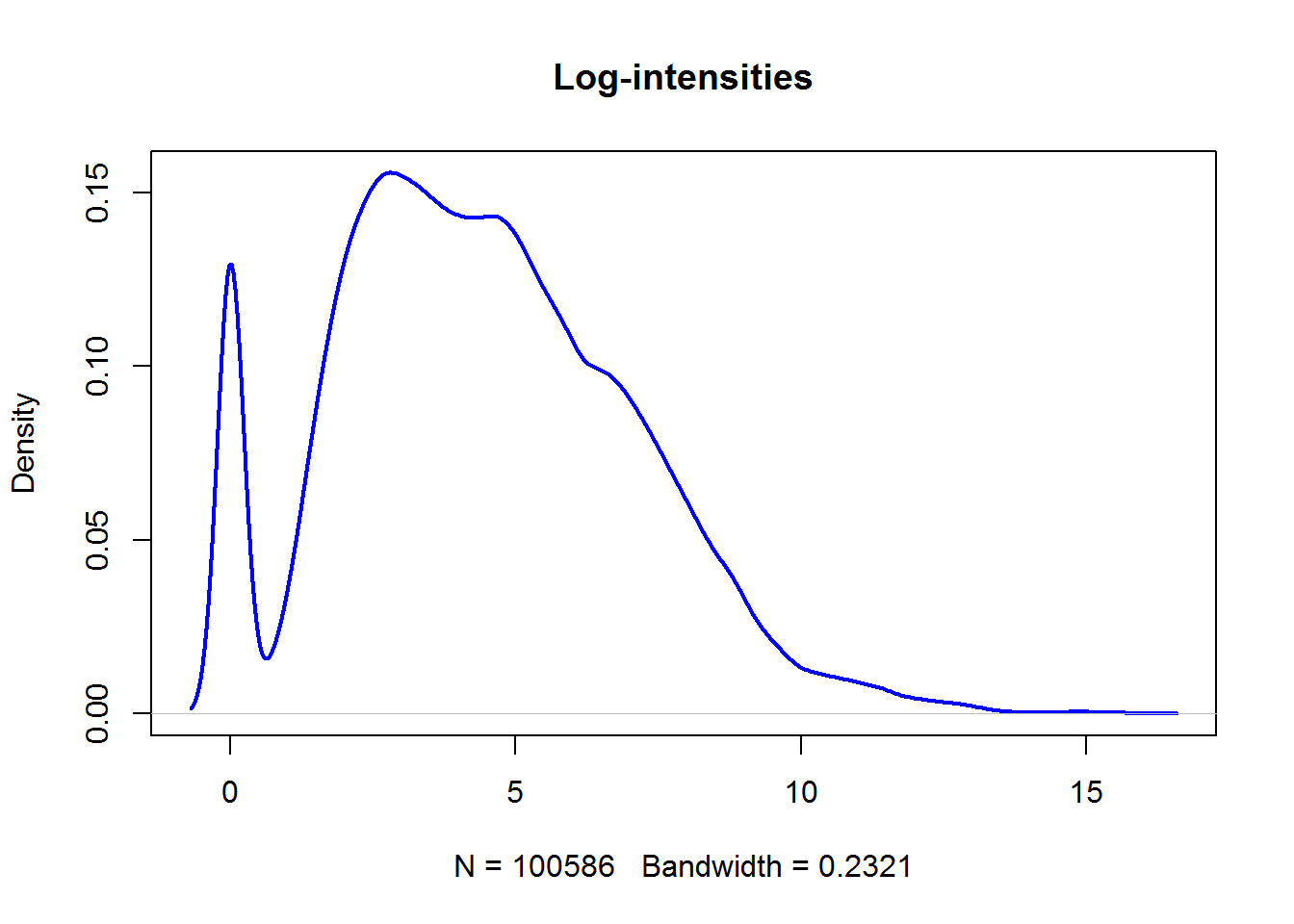
Additional functions and parameters:
legend()- adds legend to the existed plotabline()- adds a line to plot (horizontal, vertical ot tilted)pch- code of the point. See help?parfor all basic graphical parameterslwd- width of the linelty- line type (solid, dotted, etc)
2.3. Distributions of individual samples
So far we shown entire dataset as a single distribution. How about distributions for each sample individualy? One can use ggplot package or for-loop to visulaize several plots on one canvas. Let’s use custom plotDataPDF() for this.
source("http://sablab.net/scripts/plotDataPDF.r")
plotDataPDF(Data$LX,col=color,ylim=c(0,0.16))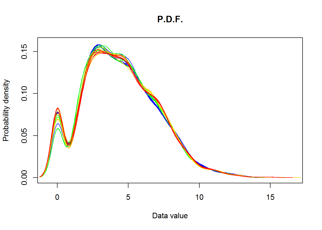
![]()