4. Clustering

4.1. The task of clustering

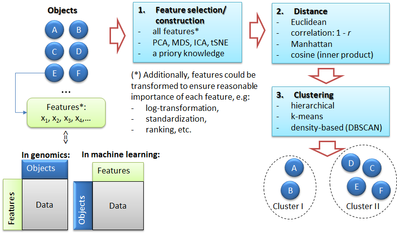
The task of clustering: (1) feature selection, (2) distance estimation, (3) unsupervised grouping - clustering

4.2. k-Means clustering

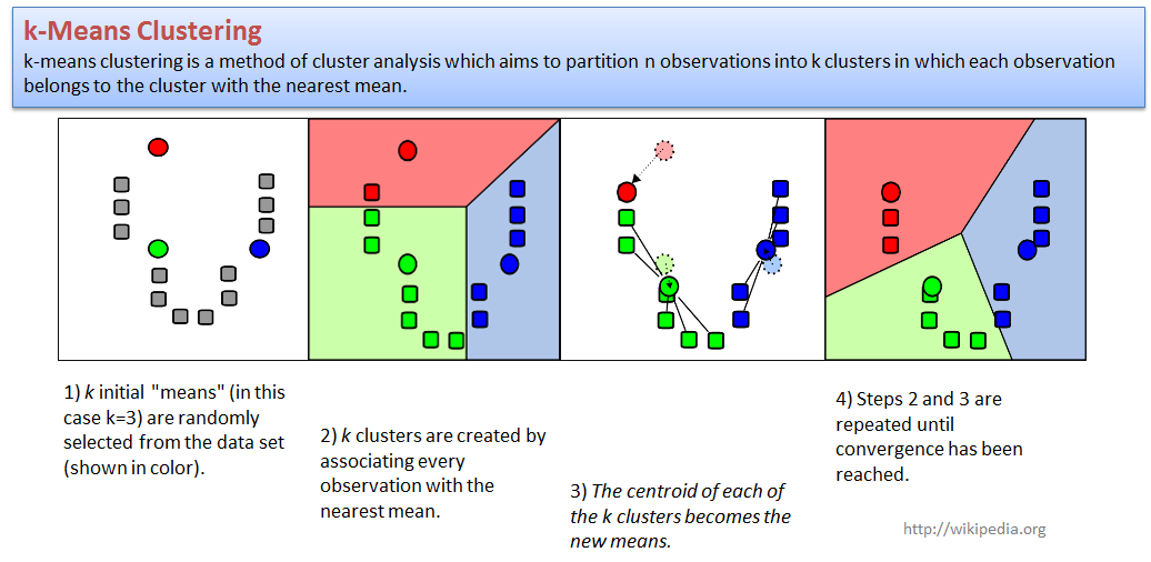
k-Means clustering - a simple and robust approach.

Let us try to cluster samples from previously considered datasets. We will use PCA to present samples in 2D space. We will use default kmeans function to cluster.

PC = prcomp(t(Data$LX),scale=TRUE) 
plot(PC$x[,"PC1"],PC$x[,"PC2"],col=1,pch=19,cex=2, main="Samples in PC-space")

## clustering -> 4 clusters
cl = kmeans(t(Data$LX),centers=4,nstart=10)$cluster
plot(PC$x[,"PC1"],PC$x[,"PC2"],col=cl+1,pch=19,cex=2, main="Samples in PC-space")

Try to change number of clusters. We can also cluster features - usually not very interesting.

cl2 = kmeans(Data$LX,centers=4,nstart=10)$cluster
plotPCA(t(Data$LX),col=cl2+1, cex=size)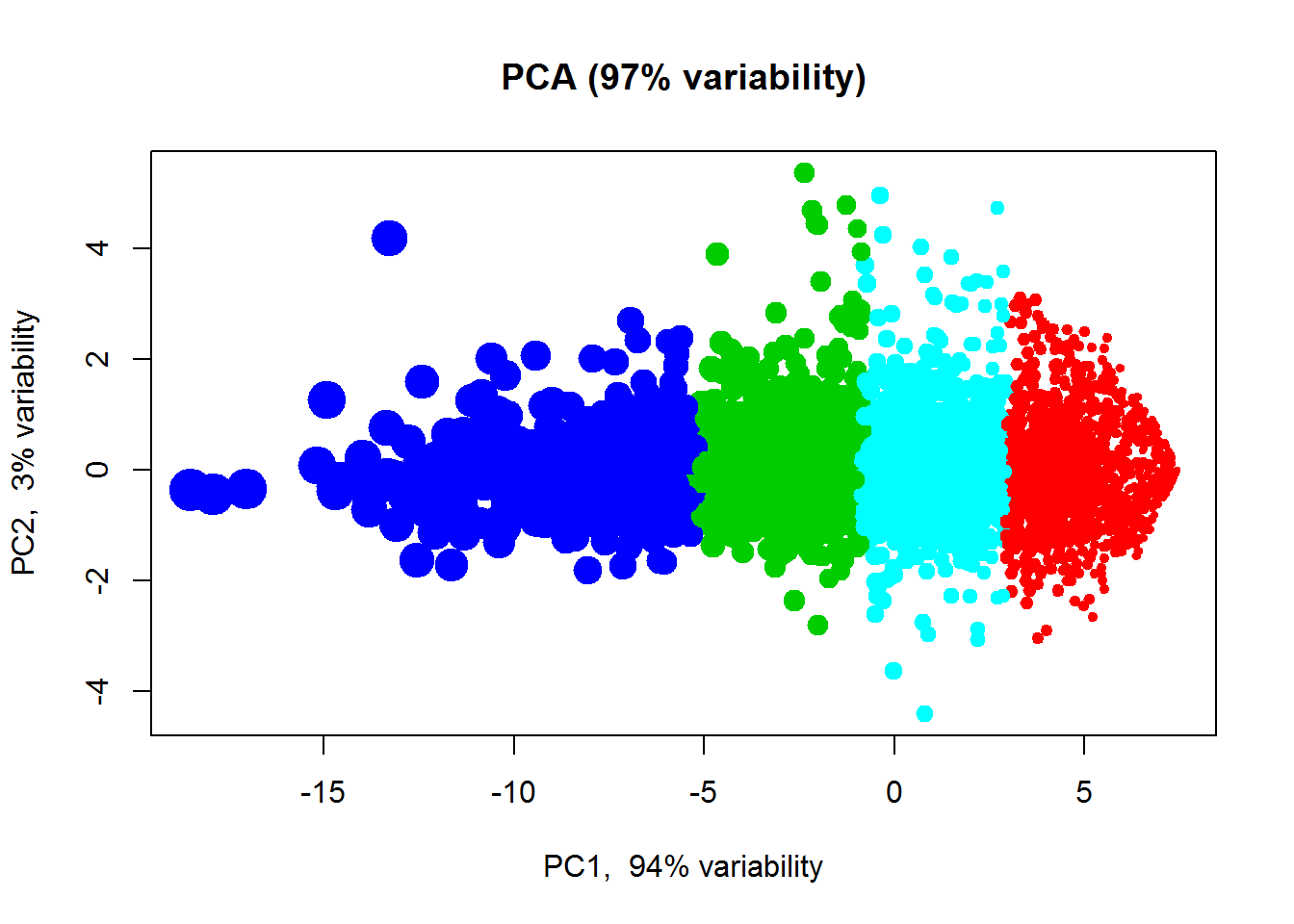

4.3. Hierarchical clustering

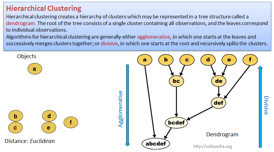
Hierarchical clustering - more flexible but less robust approach

## clustering of the samples
hc = hclust(dist(t(Data$LX)))
plot(hc)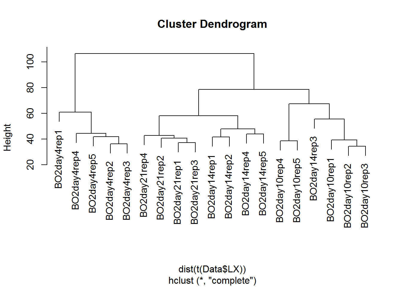

## "cut the tree" to get defined clusters
cl = cutree(hc,k=4)
plot(PC$x[,"PC1"],PC$x[,"PC2"],col=cl+1,pch=19,cex=2, main="Samples in PC-space")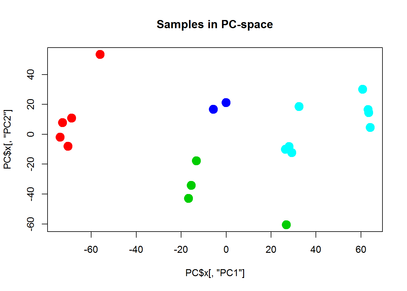

## play with k

As you can see - not so beautiful. Usually people apply consensus clustering to get defined and robust clusters.

## install the package if needed:
#install.packages("ConsensusClusterPlus")
library(ConsensusClusterPlus)
## clustering of the samples
hc = ConsensusClusterPlus(Data$LX,maxK=4,reps=100,pItem=0.8,pFeature=1, title="GeneProCC_hc",clusterAlg="hc",distance="euclidean",seed=1234567890,plot="png")
## get clusters
cl=hc[[4]]$consensusClass
## plot
plot(PC$x[,"PC1"],PC$x[,"PC2"],col=cl+1,pch=19,cex=2, main="Samples in PC-space")

Not much better but at least it is more reproducible.

4.4. Heatmaps

One of the most used methods for visualizing omics data is heatmap. Here we will use heatmaps from the package pheatmap.

## install "pheatmap" if needed
#install.packages("pheatmap")
library(pheatmap)

## Warning: package 'pheatmap' was built under R version 3.5.2

## let's use previously defined markers
pheatmap(Data$LX[imarker,], annotation_col = Data$Meta)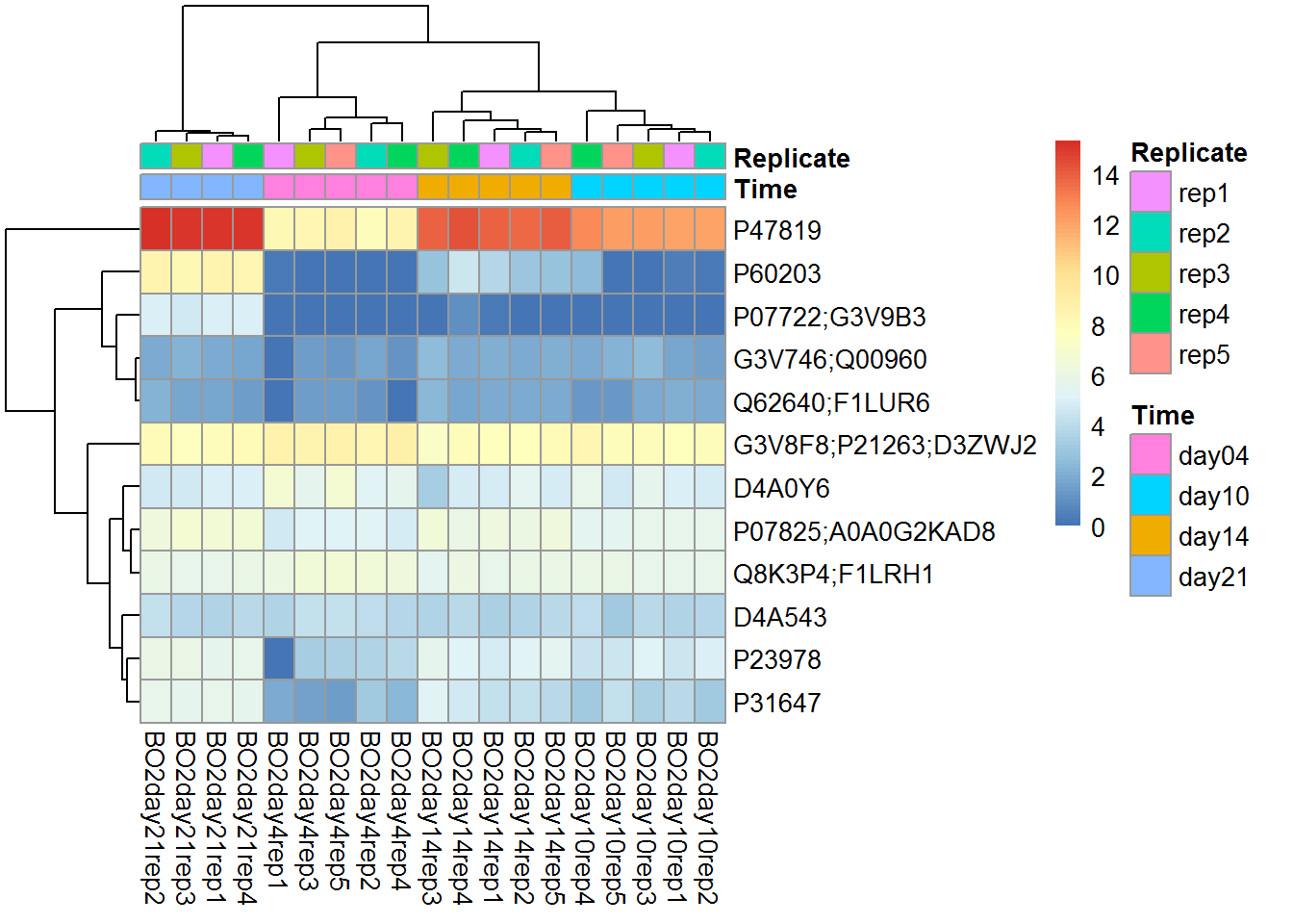

There is not much sense to build heatmaps on all available features. Let’s select the most interesting. We will use custom warp-up for Limma package: DEA.limma described in Transcriptomics course (section 4).

## load analysis function
source("http://sablab.net/scripts/LibDEA.r")
## Perform differential expression analysis (Fisher statistics)
Res = DEA.limma(Data$LX, group=Data$Meta$Time)

## Loading required package: limma

## [1] "day10-day04" "day14-day04" "day14-day10" "day21-day04" "day21-day10"
## [6] "day21-day14"
## 
## Limma,unpaired: 3619,2971,2281,1732 DEG (FDR<0.05, 1e-2, 1e-3, 1e-4)

## Significant protein groups
isig = which(Res$FDR<0.1e-4)
## reannotate features by gene names
X = Data$LX[isig,]
rownames(X) = substr(Data$Anno$Gene.names[isig],1,20)
## vizualize
pheatmap(X,scale = "row", annotation_col = Data$Meta,fontsize_row = 2)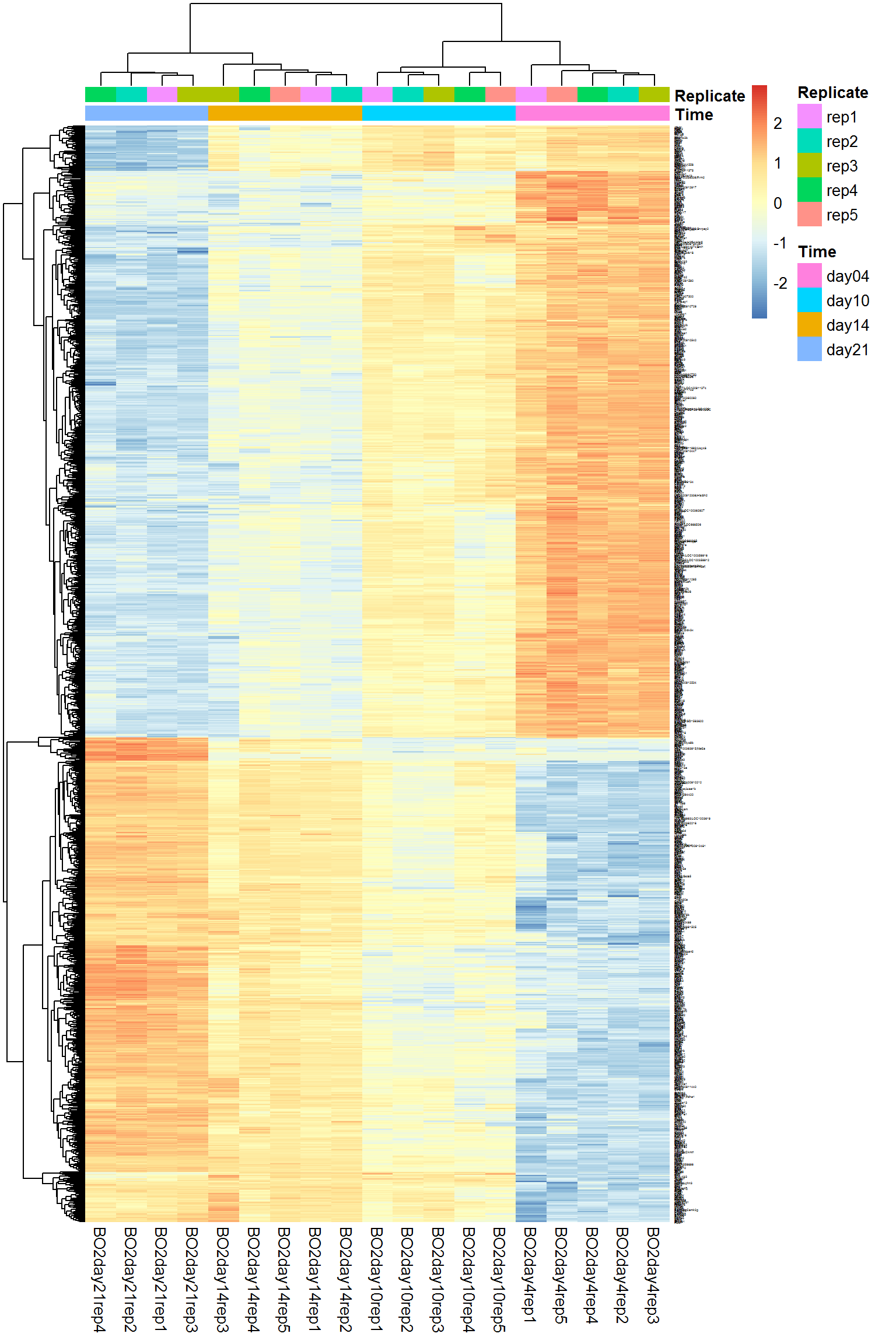