- Tutorial on Clustering
Petr V. Nazarov, LIH
2018-08-13
2.1. Installation of the required packages
Additional packages can be installed using install.packages() function in R. However it requires manual selection of the repositories that are scanned to find the package. Alternative is to use Bioconductor - it takes into account the version compatibility is usually more robust. Try:
source("https://bioconductor.org/biocLite.R")
biocLite(c("pheatmap","ConsensusClusterPlus","factoextra","NbClust","dbscan"))
2.2. Dataset import & vizualization
We will work with time-series experiment, where stimulation effect of IFNg (interferon gamma) on A375 melanoma cell line was studied. The data were published in Nazarov et al.
Let us load the data together. We need to extract 2 matrixes: X (gene expression) and Z (standardized gene expression) removing lowly expressed and non-annotated genes.
url = "http://edu.sablab.net/data/txt/mRNAIFNg.txt"

Data = read.table(url,sep="\t",head=TRUE,as.is=TRUE)
str(Data)
## 'data.frame': 10937 obs. of 25 variables:
## $ ID : int 7892501 7892502 7892503 7892504 7892505 7892506 7892507 7892508 7892509 7892510 ...
## $ gene_assignment: chr "---" "---" "---" "---" ...
## $ GeneSymbol : chr "" "" "" "" ...
## $ RefSeq : chr "---" "---" "---" "---" ...
## $ seqname : chr "---" "---" "---" "---" ...
## $ start : int 0 0 0 0 0 0 0 0 0 0 ...
## $ stop : int 0 0 0 0 0 0 0 0 0 0 ...
## $ strand : chr "---" "---" "---" "---" ...
## $ T00.1 : num 9.21 7.64 5 8.57 7.1 ...
## $ T00.2 : num 9.18 7.89 5.28 8.8 7.14 ...
## $ T03.1 : num 9.03 7.68 5.31 8.52 7.08 ...
## $ T03.2 : num 9.79 7.86 5.46 8.26 7.51 ...
## $ T12.1 : num 9.03 7.74 4.93 8.32 7.7 ...
## $ T12.2 : num 9.3 7.13 4.96 7.64 6.85 ...
## $ T24.1 : num 8.47 8 4.75 8.33 7.93 ...
## $ T24.2 : num 9.82 7.58 5.37 8.88 7.47 ...
## $ T24.3 : num 8.07 7.22 5.68 8.37 7.03 ...
## $ T48.1 : num 8.71 7.08 5.26 7.73 8.23 ...
## $ T48.2 : num 9.41 7.46 5.1 8.68 7.56 ...
## $ T48.3 : num 8.59 7.51 5.17 7.78 7.03 ...
## $ T72.1 : num 10.32 7.35 5.19 8.87 7.58 ...
## $ T72.2 : num 9.76 7.22 5.22 8.81 7.96 ...
## $ T72.3 : num 8.57 7.11 5.56 8.08 7.21 ...
## $ T72J.1 : num 9.66 8.01 5.11 8.34 7.36 ...
## $ T72J.2 : num 9.11 8.12 5.17 7.84 7.19 ...## Columns with expression start with "T" followed by the number
X = as.matrix(Data[,grep("^T[0-9]",names(Data))])
## Keep only expressed (at least once) and annotated genes
ikeep = apply(X,1,max)>5 & Data$GeneSymbol!=""
X = X[ikeep,]
rownames(X) = Data$GeneSymbol[ikeep]
str(X)## num [1:4810, 1:17] 8.8 4.8 9.47 7.78 5.52 ...
## - attr(*, "dimnames")=List of 2
## ..$ : chr [1:4810] "SEPT14" "OR4F16" "GPAM" "LOC100287934" ...
## ..$ : chr [1:17] "T00.1" "T00.2" "T03.1" "T03.2" ...## standardize expression and create matrix Z using scale() function
Z = X
Z[,] = t(scale(t(X)))
str(Z)## num [1:4810, 1:17] -0.865 -0.95 1.055 -0.249 0.163 ...
## - attr(*, "dimnames")=List of 2
## ..$ : chr [1:4810] "SEPT14" "OR4F16" "GPAM" "LOC100287934" ...
## ..$ : chr [1:17] "T00.1" "T00.2" "T03.1" "T03.2" ...Now we can define time-groups of the samples and start vizualizing using PCA. Let’s perform several PCAs:
- PCSX - PCA using samples as objects, unscaled data X
- PCSZ - PCA using samples as objects, centered/scaled data Z
- PCGX - PCA using genes as objects, unscaled data X
- PCGZ - PCA using genes as objects, centered/scaled data Z
## groups and colors
group = factor(sub("[.].+","",colnames(X)))
color = rainbow(nlevels(group))[as.integer(group)]
names(color) = colnames(X)

## PCSX - PCA using Samples as
PCSX = prcomp(t(X))
PCSZ = prcomp(t(Z))
PCGX = prcomp(X)
PCGZ = prcomp(Z)

plot(PCSX$x[,1],PCSX$x[,2],col=color,pch=14 + as.integer(group),cex=2, main="PCA of Samples, unscaled")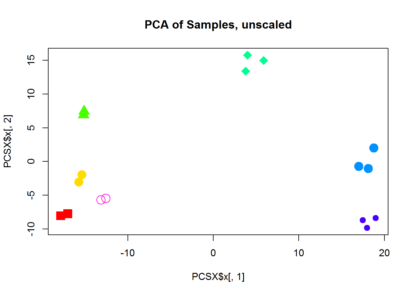
plot(PCSZ$x[,1],PCSZ$x[,2],col=color,pch=14 + as.integer(group),cex=2, main="PCA of Samples, centered/scaled")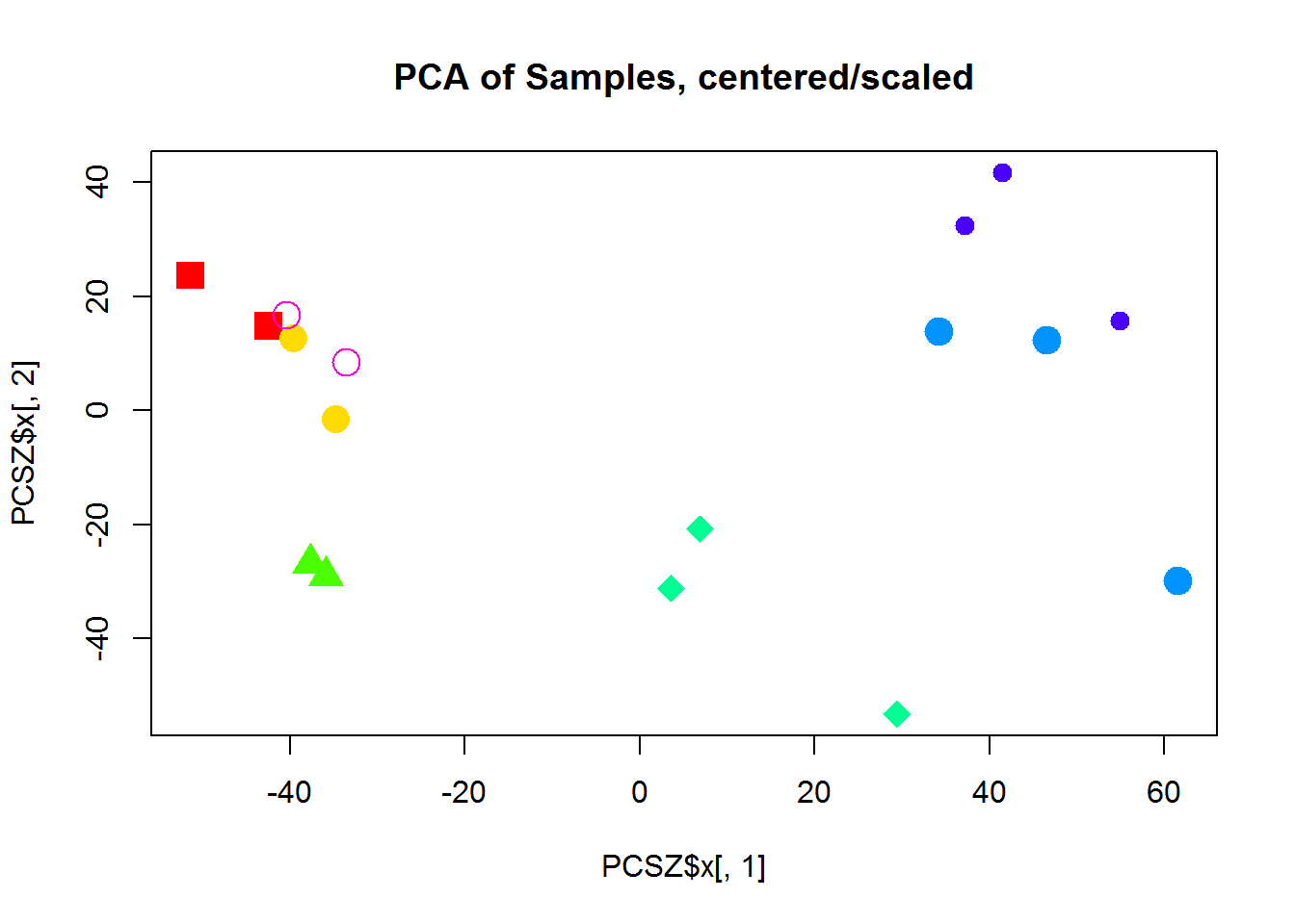
plot(PCGX$x[,1],PCGX$x[,2],col="#0000FF55",pch=19,main="PCA of Genes, unscaled")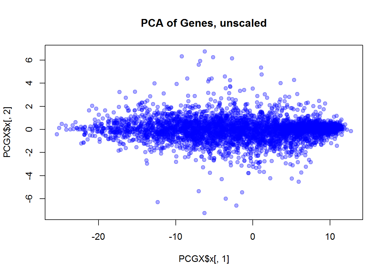
plot(PCGZ$x[,1],PCGZ$x[,2],col="#0000FF55",pch=19,main="PCA of Genes, centered/scaled")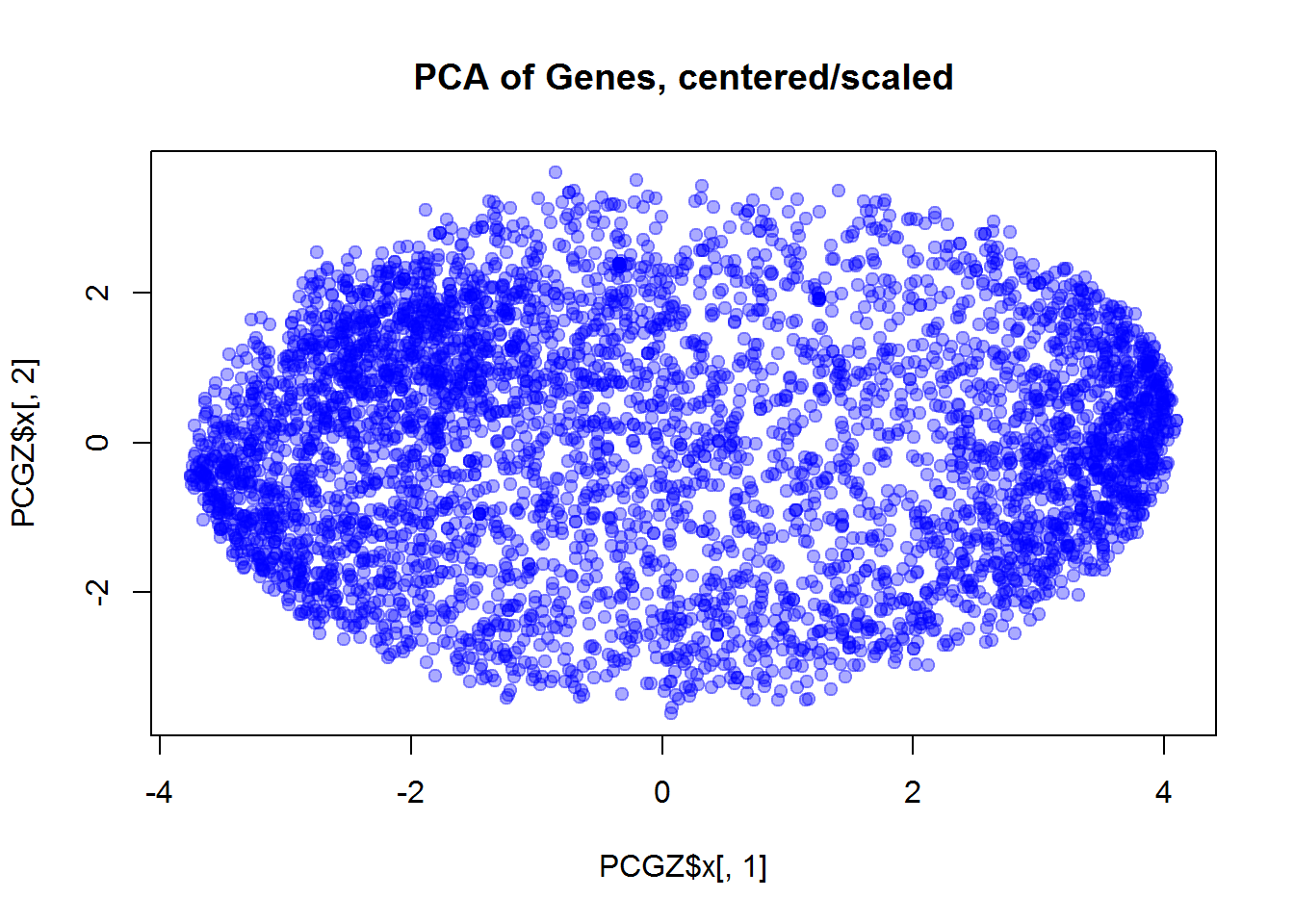
Independent work: please try to answer the questions using code presented in the lecture and reproduce the results shown below
2.3. Cluster the samples
2.3.1. Hierarchical clustering
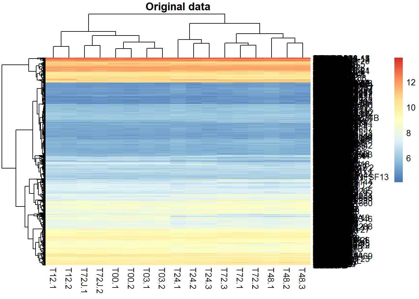
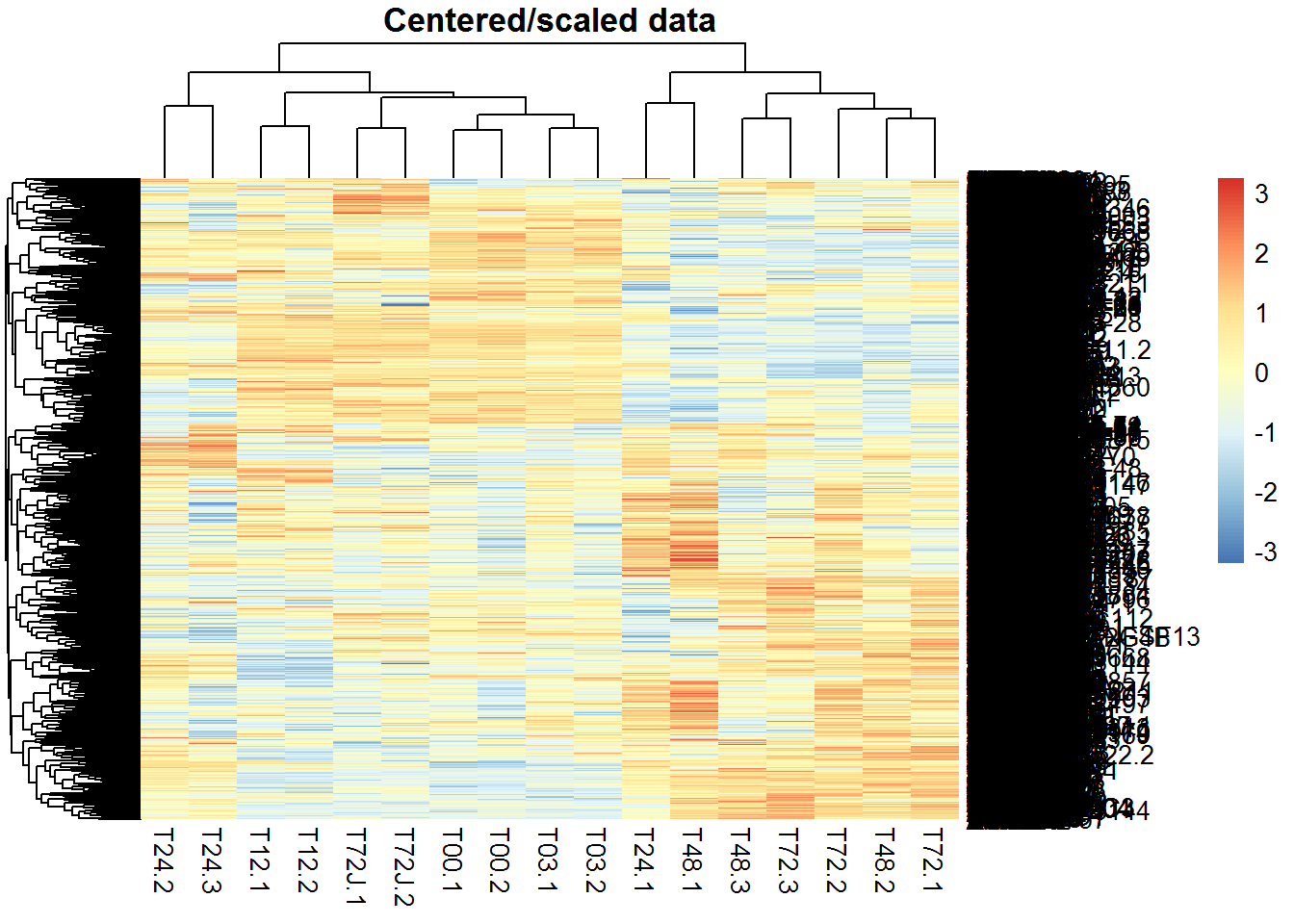
Let’s build bi-clusters of genes and samples. Use 2 variants: X and Z. Load the library using library(pheatmap). Alternatively the simple heatmap() can be used (though it is much slower).
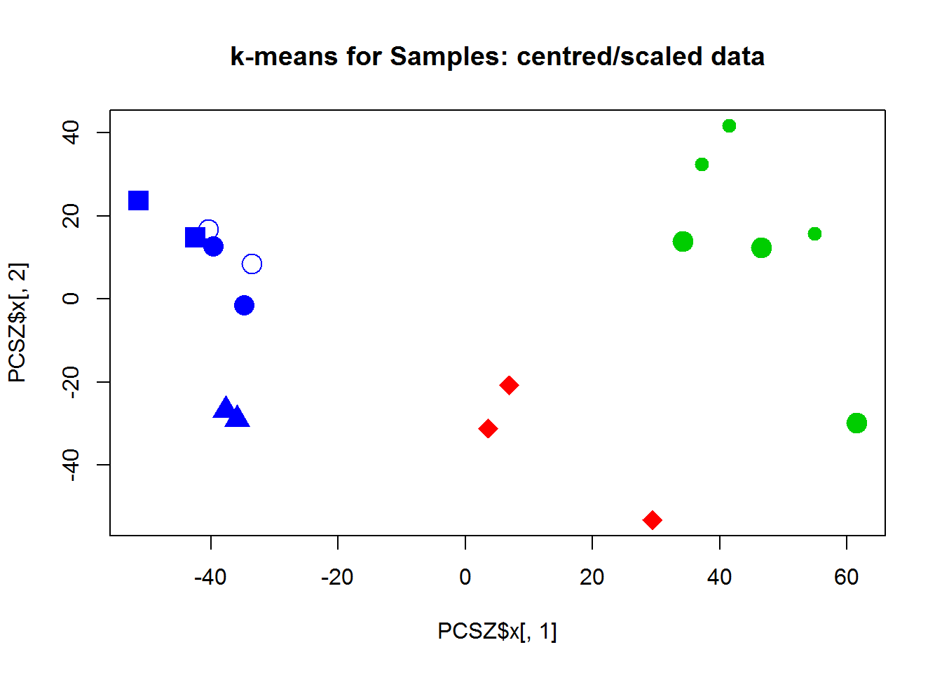
2.3.2. Non-hierarchical clustering of samples
Now let’s use k-means or PAM to cluster the samples. Hint: if you use X with genes in rows, you should transpose it: kmeans(t(X),centers=3) For 3 clusters we have:
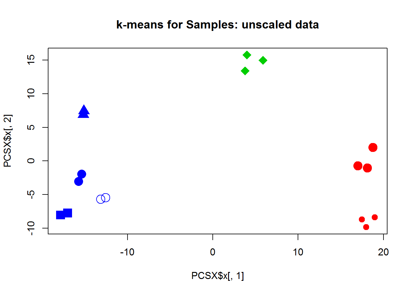
## cl
## group 1 2 3
## T00 0 0 2
## T03 0 0 2
## T12 0 0 2
## T24 3 0 0
## T48 0 3 0
## T72 0 3 0
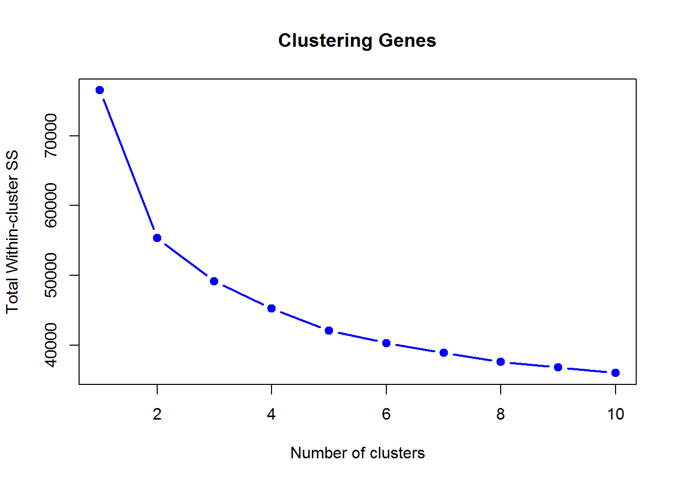
## T72J 0 0 2Here is WSS decrease with the number of clusters (unscaled data X):
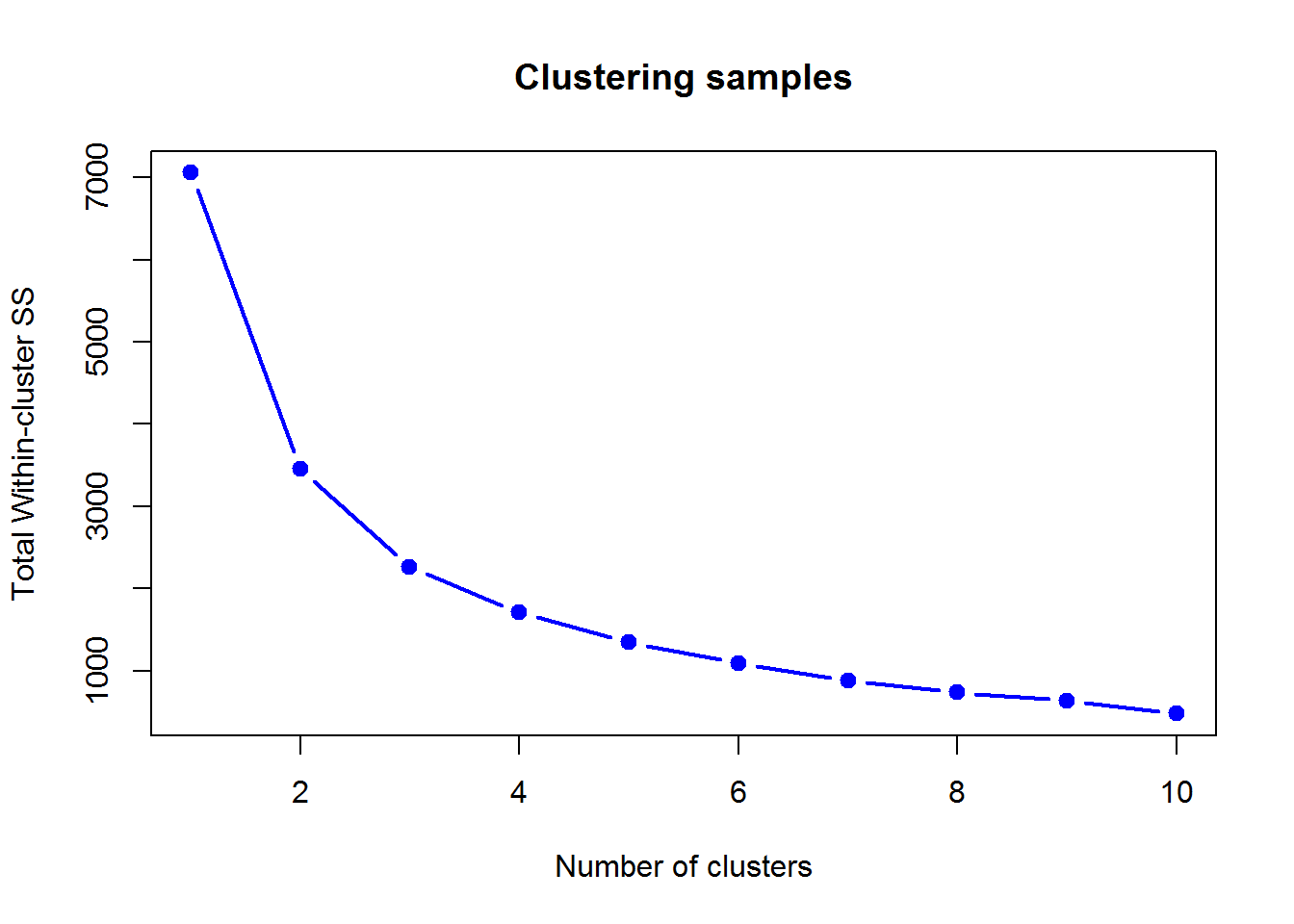
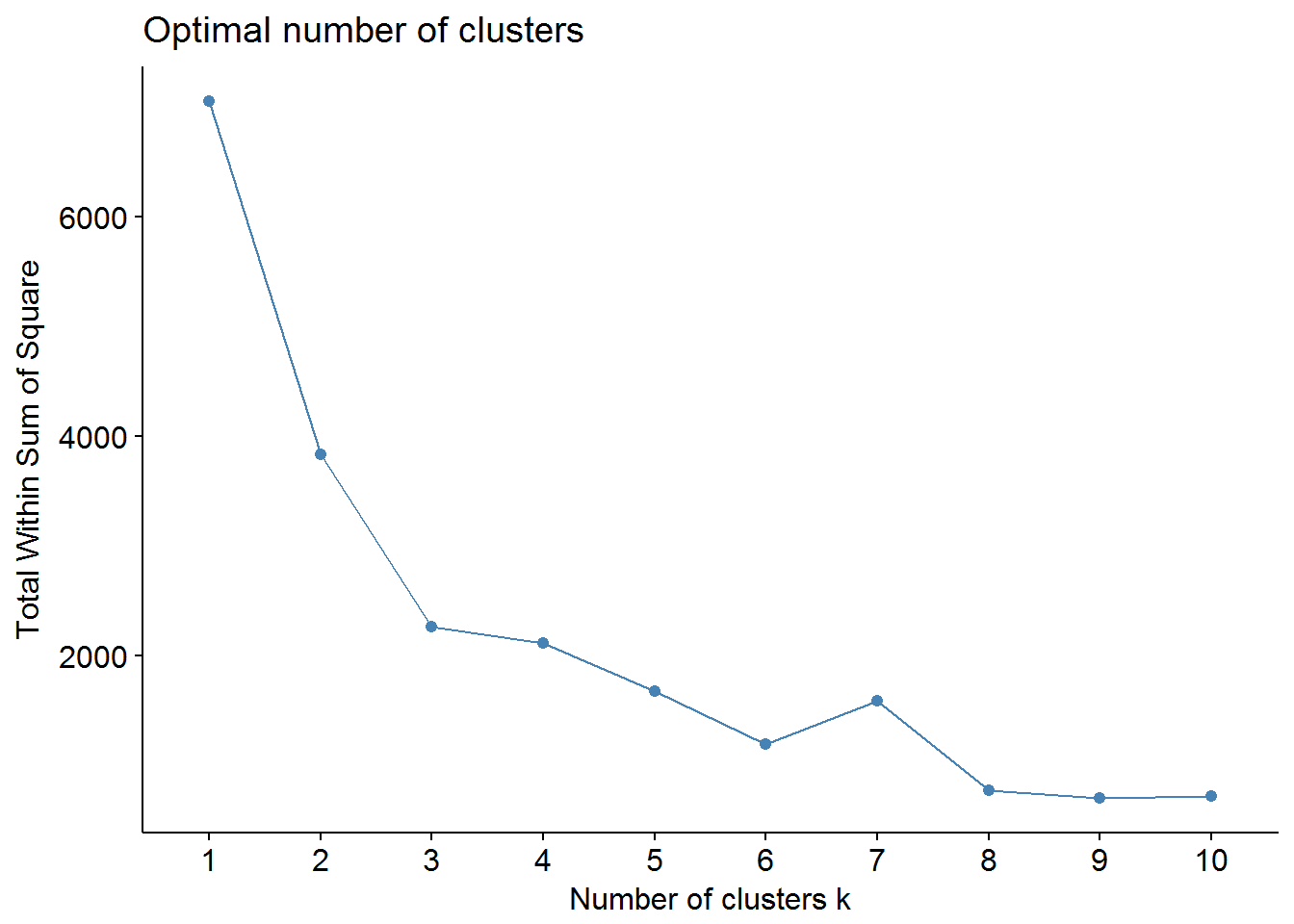
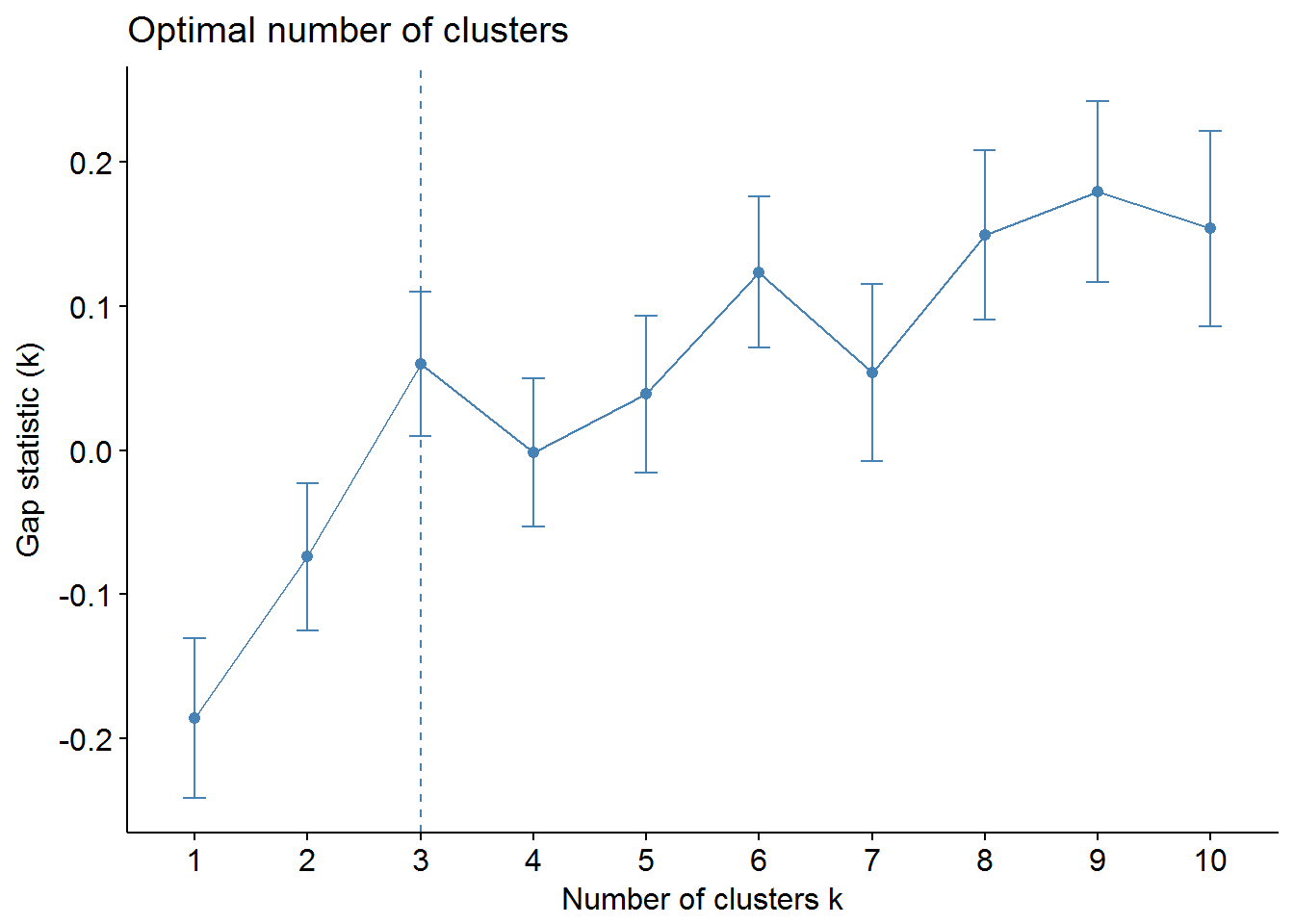
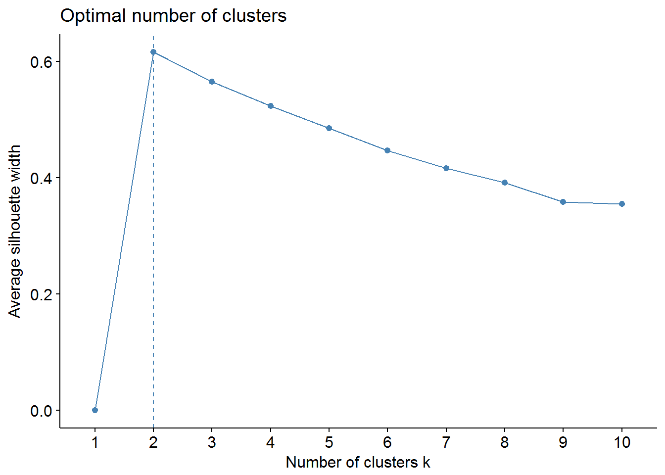
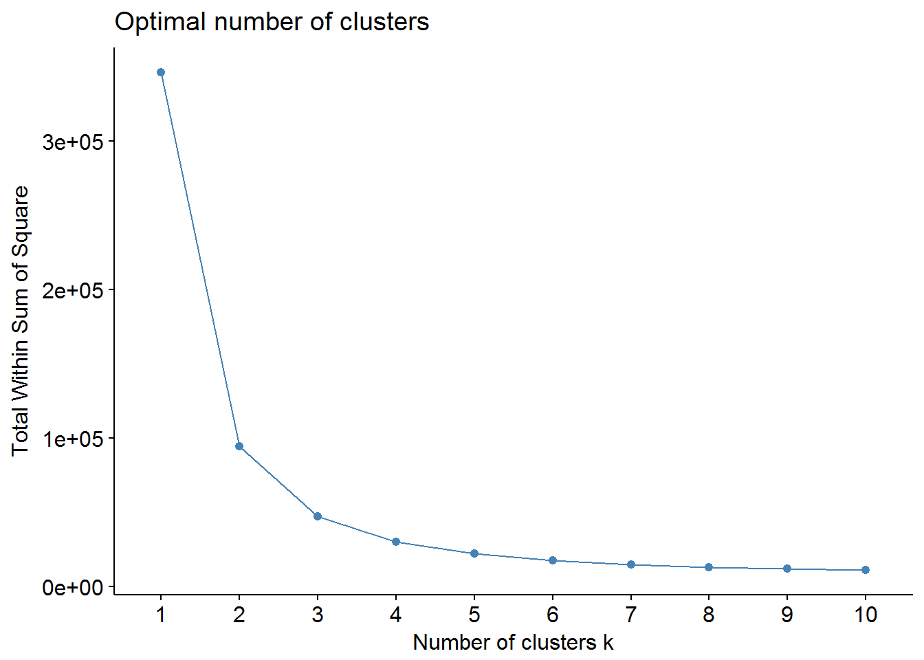
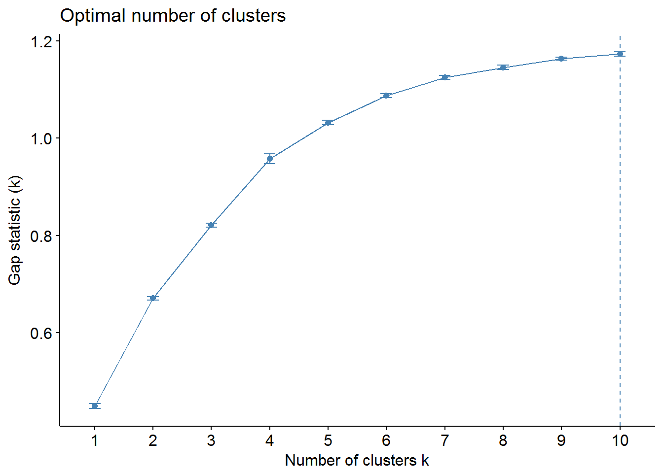
We can use factoextra and NbClust packages to find out the optimal number of clusters
## Warning: package 'factoextra' was built under R version 3.4.4## Loading required package: ggplot2## Welcome! Related Books: `Practical Guide To Cluster Analysis in R` at https://goo.gl/13EFCZ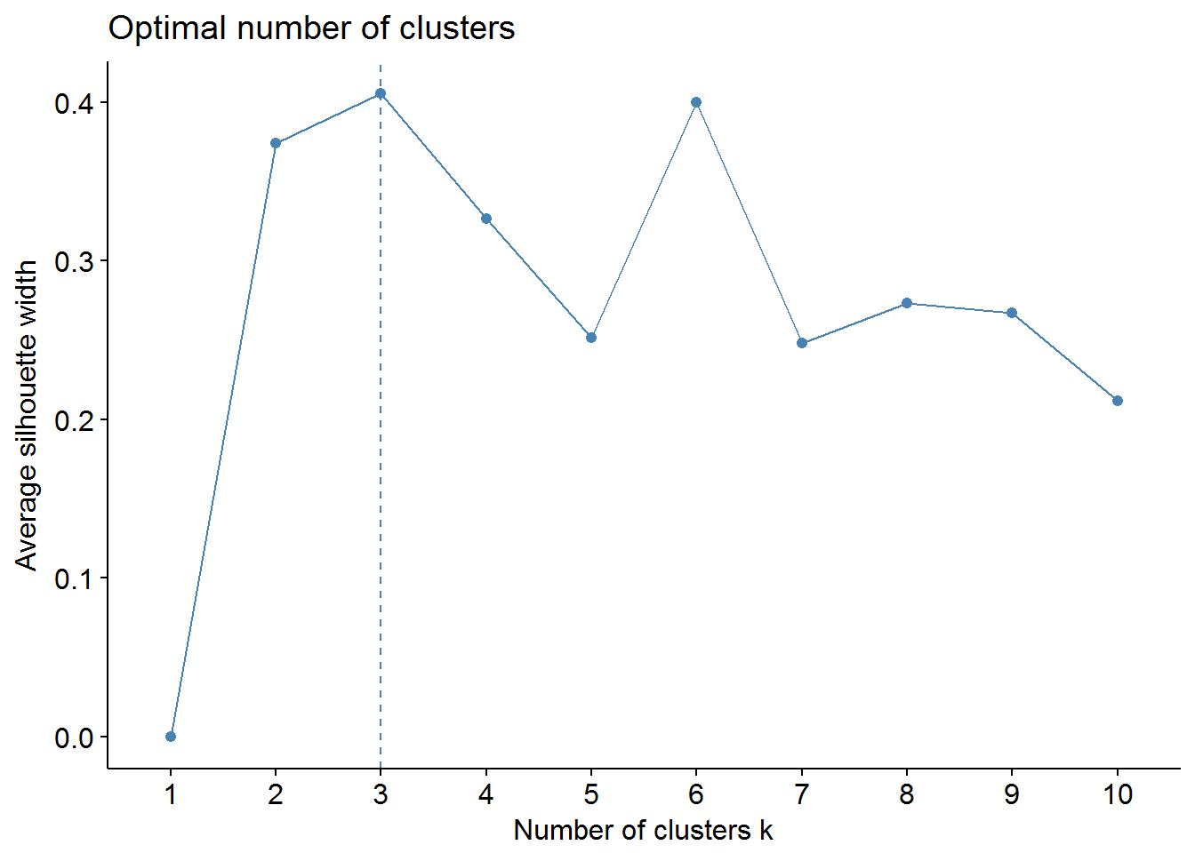
2.3.2. Non-hierarchical clustering of genes
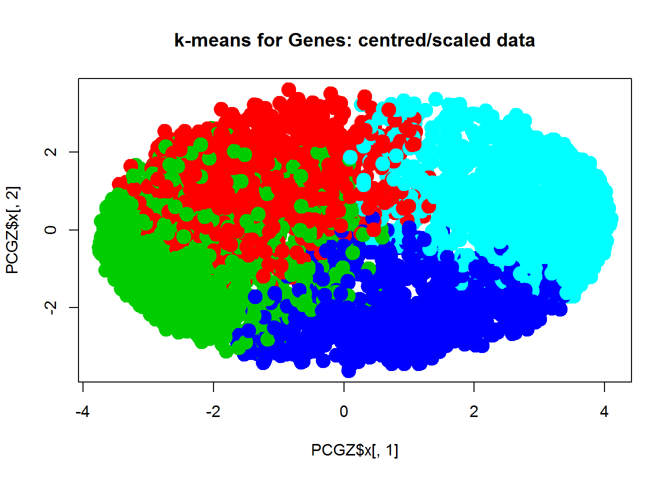
![]()