- Data Analysis in Single Cell Transcriptomics
Petr V. Nazarov, LIH
2018-08-14
3.1. ICA & PCA
Let’s see how ICA can be used for data vizualization and compare with PCA. For simplisity - used IRIS dataset :)
X = t(as.matrix(iris[,-5]))
color = as.integer(iris[,5])

PC = prcomp(t(X))
x1.lim=c(1.2*min(PC$x[,1]),1.2*max(PC$x[,1]));x2.lim=c(1.2*min(PC$x[,2]),1.2*max(PC$x[,2]))
plot(PC$x[,1],PC$x[,2], col=color,pch=19,cex=1, xlim=x1.lim, ylim=x2.lim,
    main=sprintf("PCA (%d%% variability)", round((PC$sdev[1]^2+PC$sdev[2]^2)/sum(PC$sdev^2)*100)),cex.main=1,
    ylab=sprintf("PC2, includes %d%% variability",round(PC$sdev[2]^2 /sum(PC$sdev^2)*100)),
    xlab=sprintf("PC1, includes %d%% variability",round(PC$sdev[1]^2 /sum(PC$sdev^2)*100)))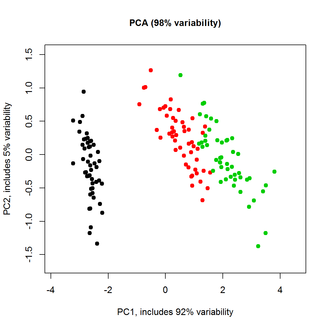
str(PC)## List of 5
## $ sdev : num [1:4] 2.056 0.493 0.28 0.154
## $ rotation: num [1:4, 1:4] 0.3614 -0.0845 0.8567 0.3583 -0.6566 ...
## ..- attr(*, "dimnames")=List of 2
## .. ..$ : chr [1:4] "Sepal.Length" "Sepal.Width" "Petal.Length" "Petal.Width"
## .. ..$ : chr [1:4] "PC1" "PC2" "PC3" "PC4"
## $ center : Named num [1:4] 5.84 3.06 3.76 1.2
## ..- attr(*, "names")= chr [1:4] "Sepal.Length" "Sepal.Width" "Petal.Length" "Petal.Width"
## $ scale : logi FALSE
## $ x : num [1:150, 1:4] -2.68 -2.71 -2.89 -2.75 -2.73 ...
## ..- attr(*, "dimnames")=List of 2
## .. ..$ : NULL
## .. ..$ : chr [1:4] "PC1" "PC2" "PC3" "PC4"
## - attr(*, "class")= chr "prcomp"library(fastICA)
IC = fastICA(X,n.comp=2,alg.typ ="deflation")
plot(IC$A[1,],IC$A[2,], col=color,pch=19,cex=1, main="ICA",cex.main=1,ylab="IC2", xlab="IC1")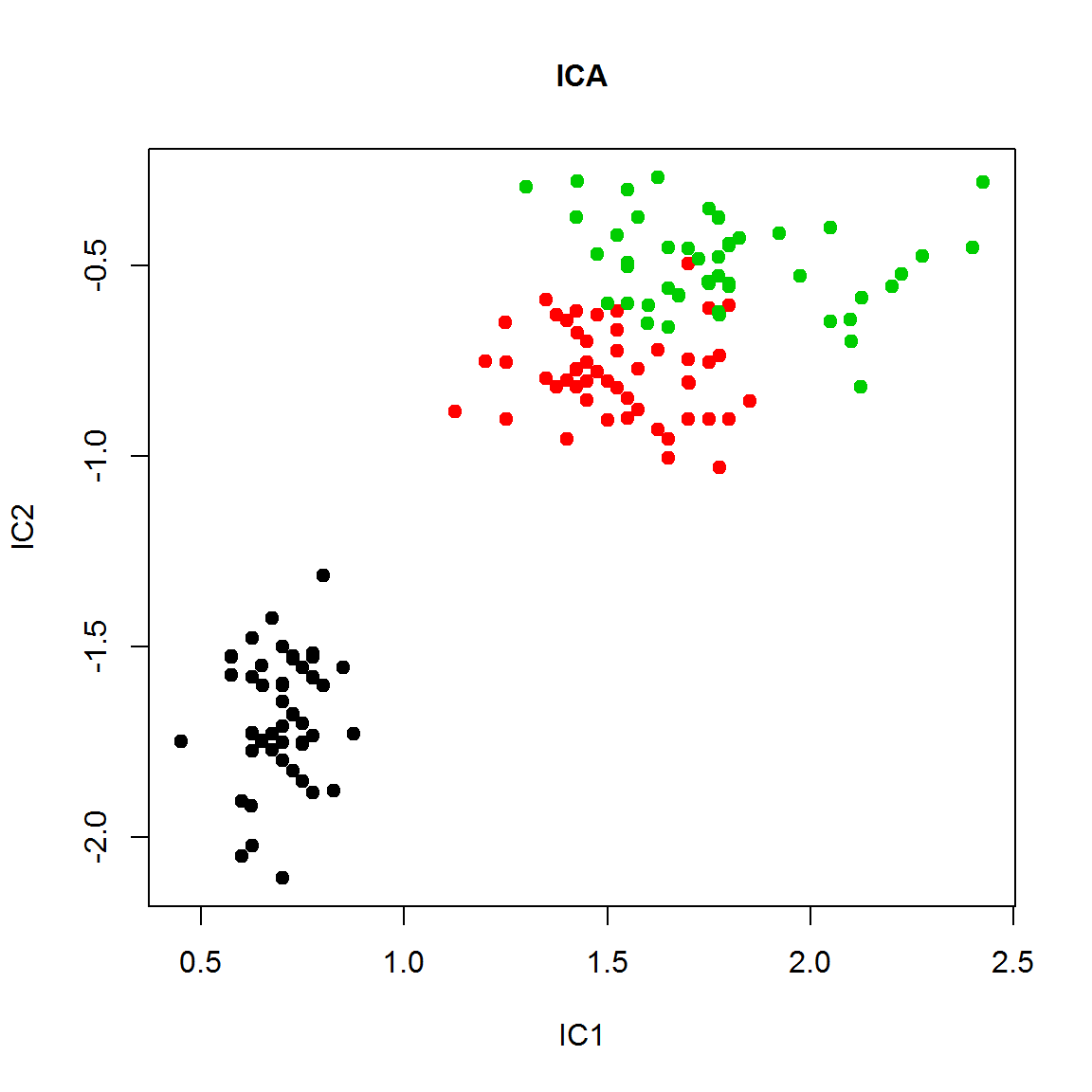
## Note: for more robust decomposition - use consensus ICA function runICA() from
## source("http://sablab.net/scripts/LibICA.r")
3.2. tSNE
Let’s try using tSNE on iris dataset. See the difference b/w PCA and tSNE with various perplexity parameter.
library(tsne)
species = iris$Species
color = as.integer(species)    ## for the moment let's color by species
point = 14+as.integer(species) ## point shape will represent species

X = as.matrix(iris[,-5])
PC = prcomp(X)
plot(PC$x[,1],PC$x[,2],col=color,pch=point)
legend("topright",legend=levels(species), pch=unique(point))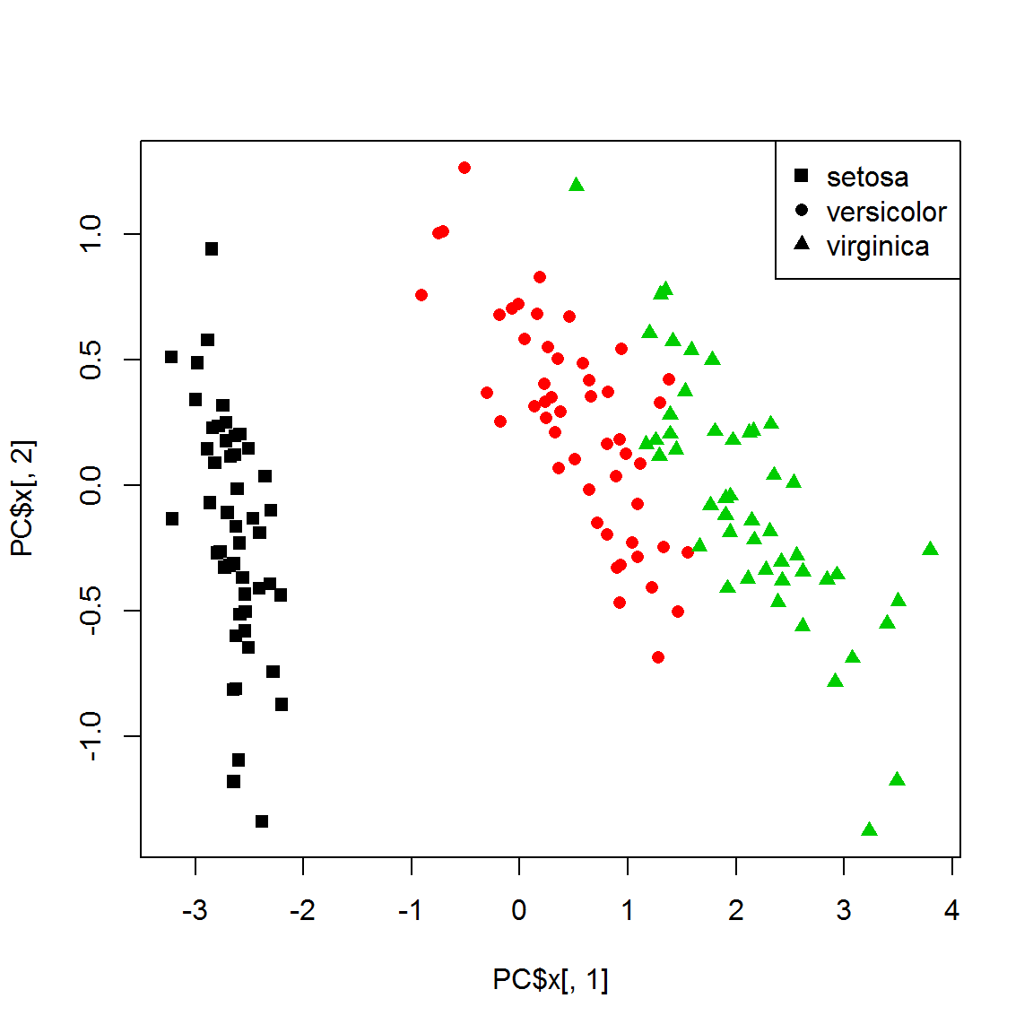
par(mfrow=c(2,2))
TS = tsne(X, perplexity = 5, max_iter = 500,epoch=100)
## sigma summary: Min. : 0.214997645851654 |1st Qu. : 0.342847116876516 |Median : 0.37968157669647 |Mean : 0.393228519246909 |3rd Qu. : 0.432601154083186 |Max. : 0.642443927774078 |## Epoch: Iteration #100 error is: 15.6567462140163## Epoch: Iteration #200 error is: 2.44899177660879## Epoch: Iteration #300 error is: 2.69311816826899## Epoch: Iteration #400 error is: 2.24104464414752## Epoch: Iteration #500 error is: 2.13318812818345plot(TS[,1],TS[,2], pch = point, col=color,main="Perplexity = 5")
TS = tsne(X, perplexity = 20, max_iter = 500,epoch=100)## sigma summary: Min. : 0.42864778740551 |1st Qu. : 0.523593962475894 |Median : 0.553545139847788 |Mean : 0.563823813379956 |3rd Qu. : 0.596877396756174 |Max. : 0.752227354673175 |## Epoch: Iteration #100 error is: 13.7384706201221## Epoch: Iteration #200 error is: 0.29085053861169## Epoch: Iteration #300 error is: 0.270363430080117## Epoch: Iteration #400 error is: 0.269068675072325## Epoch: Iteration #500 error is: 0.268710639574665plot(TS[,1],TS[,2], pch = point, col=color,main="Perplexity = 20")
TS = tsne(X, perplexity = 50, max_iter = 500,epoch=100)## sigma summary: Min. : 0.565012665854053 |1st Qu. : 0.681985646004023 |Median : 0.713004330336136 |Mean : 0.716213420895748 |3rd Qu. : 0.74581655363904 |Max. : 0.874979764925049 |## Epoch: Iteration #100 error is: 12.2102603478457## Epoch: Iteration #200 error is: 0.19070861618852## Epoch: Iteration #300 error is: 0.188988578907063## Epoch: Iteration #400 error is: 0.188987986302044## Epoch: Iteration #500 error is: 0.188987986290783plot(TS[,1],TS[,2], pch = point, col=color,main="Perplexity = 50")
TS = tsne(X, perplexity = 100, max_iter = 500,epoch=100)## sigma summary: Min. : 0.776385211439336 |1st Qu. : 0.927141154386403 |Median : 0.971370883716192 |Mean : 0.961326081014028 |3rd Qu. : 0.99555893656996 |Max. : 1.09859103718956 |## Epoch: Iteration #100 error is: 10.3041970532984## Epoch: Iteration #200 error is: 0.110709369927684## Epoch: Iteration #300 error is: 0.110709359856045## Epoch: Iteration #400 error is: 0.110709359856045## Epoch: Iteration #500 error is: 0.110709359856045plot(TS[,1],TS[,2], pch = point, col=color,main="Perplexity = 100")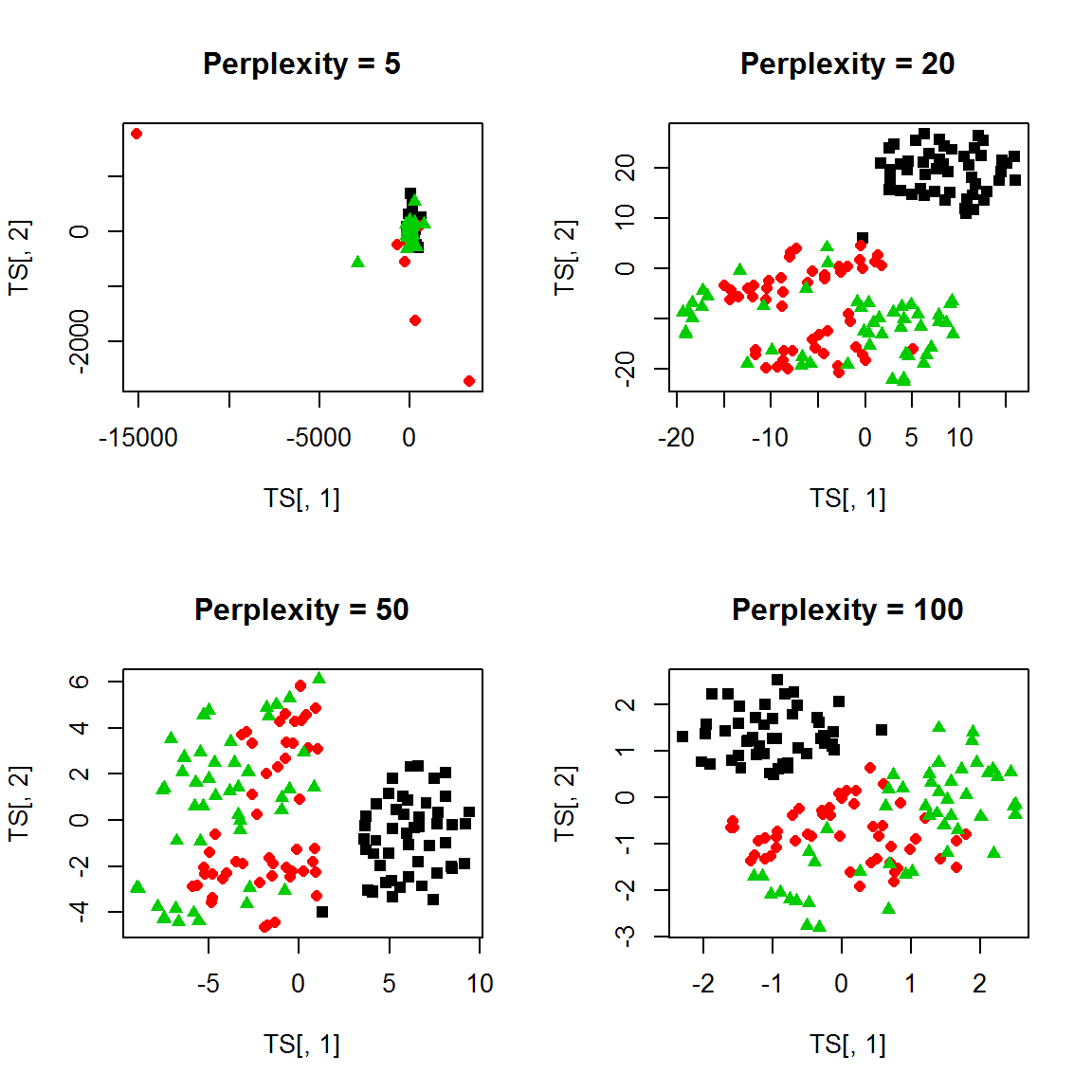
![]()