- Lecture on Clustering
Petr V. Nazarov, LIH
2018-08-13
1.1. Data preparation and initial vizualization
Let us first clean memory and setup the current folder, where our results will be stored.
rm(list=ls()) ## clean memory
gc() ## garbage collection

getwd()   # shows current folder
setwd("D:/Data/Clustering") # sets the current folder
Here we will use the standard iris dataset (R.Fisher, 1936) that is available in R by default.
str(iris)## 'data.frame': 150 obs. of 5 variables:
## $ Sepal.Length: num 5.1 4.9 4.7 4.6 5 5.4 4.6 5 4.4 4.9 ...
## $ Sepal.Width : num 3.5 3 3.2 3.1 3.6 3.9 3.4 3.4 2.9 3.1 ...
## $ Petal.Length: num 1.4 1.4 1.3 1.5 1.4 1.7 1.4 1.5 1.4 1.5 ...
## $ Petal.Width : num 0.2 0.2 0.2 0.2 0.2 0.4 0.3 0.2 0.2 0.1 ...
## $ Species : Factor w/ 3 levels "setosa","versicolor",..: 1 1 1 1 1 1 1 1 1 1 ...species = iris$Species
color = as.integer(species) ## for the moment let's color by species
point = 14+as.integer(species) ## point shape will represent species
plot(iris[,-5],pch=point, col=color)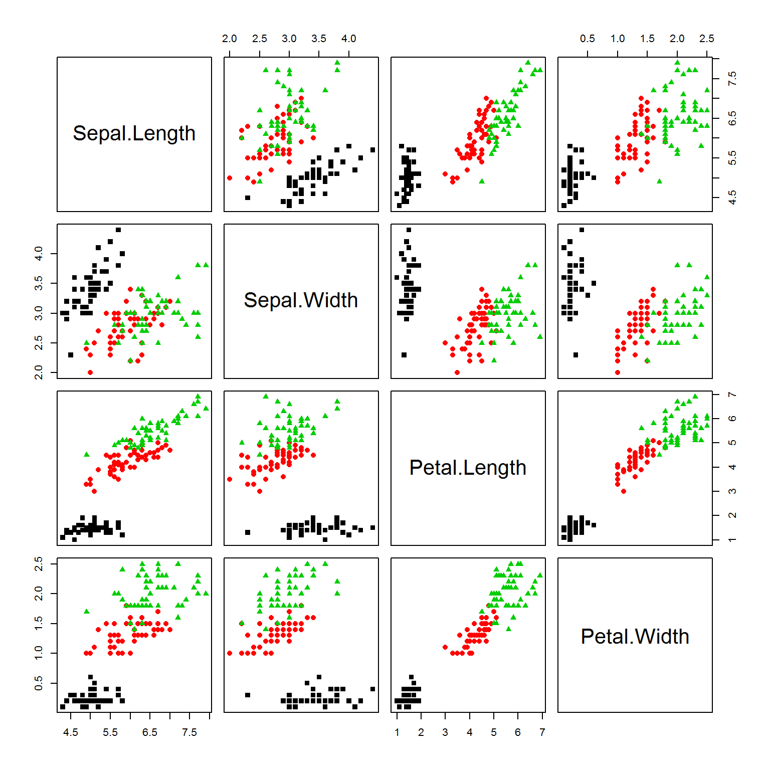
## let's extract features and scale the data
X = as.matrix(iris[,-5])
X[,] = scale(X)
Now, apply PCA to vizualize 4d data in 2d. This is the best possible representation based on variability.
PC = prcomp(X)
plot(PC$x[,1],PC$x[,2],col=color,pch=point)
legend("topright",legend=levels(species), pch=unique(point))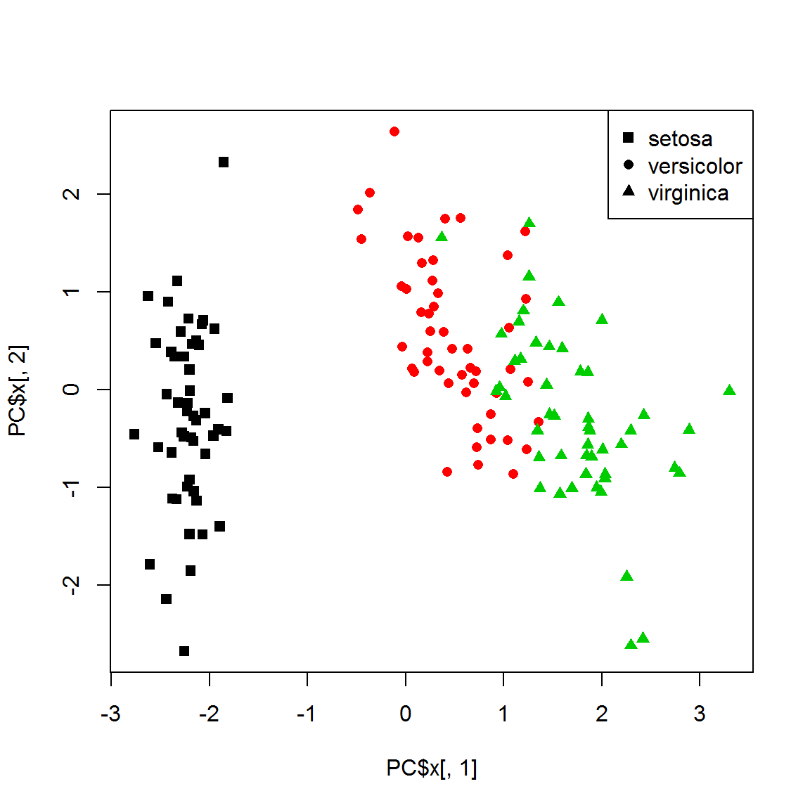
1.2. Hierarchical clustering
1.2.1. Simple hierarchical clustering
H = hclust(dist(X))
cl = cutree(H,k=3)

plot(H,labels=species,hang=-1,cex=0.75)
points(x=1:nrow(X),y=rep(0,nrow(X)),pch=point[H$order],col=cl[H$order])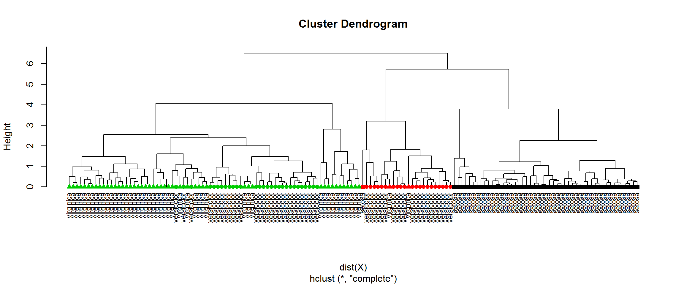
table(cl, species)## species
## cl setosa versicolor virginica
## 1 49 0 0
## 2 1 21 2
## 3 0 29 48Now let’s check the stability of such clustering by removing one flower from each group
idx = c(-41,-98,-144) ## 3 preselected objects removed
X1 = X[idx,]
color1 = color[idx]
point1 = point[idx]
species1 = species[idx]
H1 = hclust(dist(X1))
cl1 = cutree(H1,k=3)
plot(H1,labels=species1,hang=-1,cex=0.75, main="Cluster Dendrogram after Removing")
points(x=1:nrow(X1),y=rep(0,nrow(X1)),pch=point1[H1$order],col=cl1[H1$order])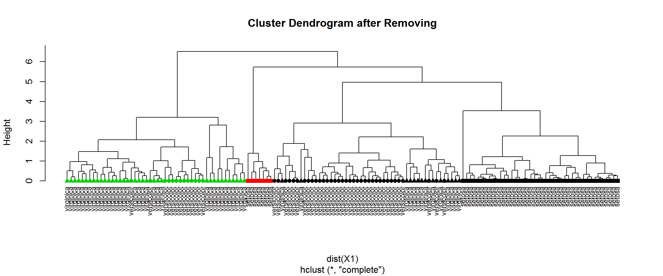
table(cl[idx],cl1) ## compare with previous clustering## cl1
## 1 2 3
## 1 41 7 0
## 2 24 0 0
## 3 27 0 48table(species1,cl1) ## compare with species groups## cl1
## species1 1 2 3
## setosa 42 7 0
## versicolor 36 0 13
## virginica 14 0 35You can easily build bi-clusters of the dataset (clusteting similar objects and similar features at the same time) using heatmap() function, or more advanced pheatmap(). Please use ?pheatmap to see what visual parameters you can control.
library(pheatmap)
pheatmap(X)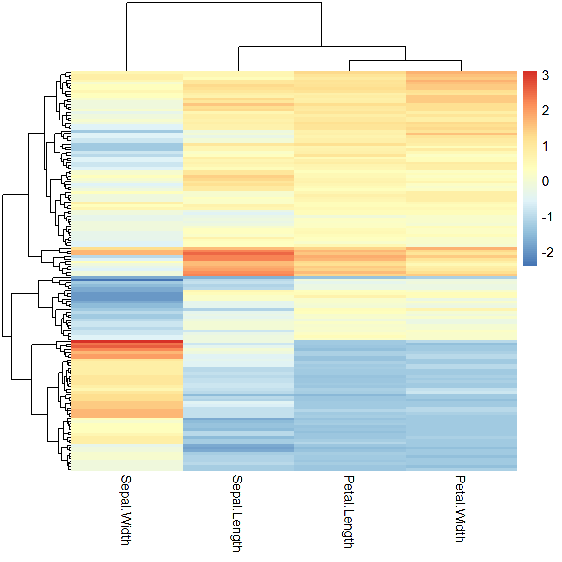
1.2.2. Other distance measures
Try using other distance measures that are implemented in dist() function:
H2 = hclust(dist(X,method="maximum"))
cl2 = cutree(H2,k=3)
table(cl2, species)
## species
## cl2 setosa versicolor virginica
## 1 37 40 20
## 2 13 0 0
## 3 0 10 30Or use your own definition of the distance, e.g. often-used correlation measure:
D = (1-cor(t(X)))/2
D = as.dist(D)
H3 = hclust(D)
cl3 = cutree(H3,k=3)
table(cl3, species)
## species
## cl3 setosa versicolor virginica
## 1 49 2 0
## 2 1 10 14
## 3 0 38 361.2.3 Consensus hierarchical clustering
Consensus HC can improve stability of clustering. Usually it is performed in 3 steps:
- Resampling of the original set
- Clustering
- Summarizing the results
However, there is no guarantee that you will get what you expect…
library(ConsensusClusterPlus)
results = ConsensusClusterPlus(t(X),maxK=6,reps=50,pItem=0.8,pFeature=1,title="IRIS ConClust",clusterAlg="hc",distance="euclidean",seed=12345,plot="png")
## end fraction## clustered
## clustered
## clustered
## clustered
## clusteredplot(PC$x[,1],PC$x[,2],col=results[[3]]$consensusClass, pch=point)
legend("topright",legend=levels(species), pch=unique(point))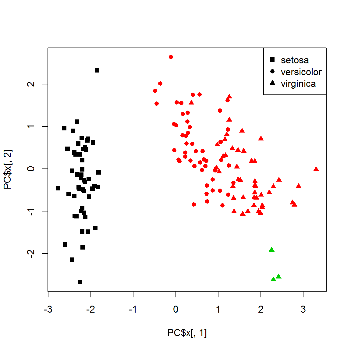
table(species, results[[3]]$consensusClass)##
## species 1 2 3
## setosa 50 0 0
## versicolor 0 50 0
## virginica 0 47 31.3. Non-hierarchical clustering
1.3.1. k-means
Widely used method of non-hierarchical clustering is k-means. You should predefine number of clusters
cl = kmeans(X,centers=3, nstart=10)$cluster
plot(PC$x[,1],PC$x[,2],col = cl,pch=point)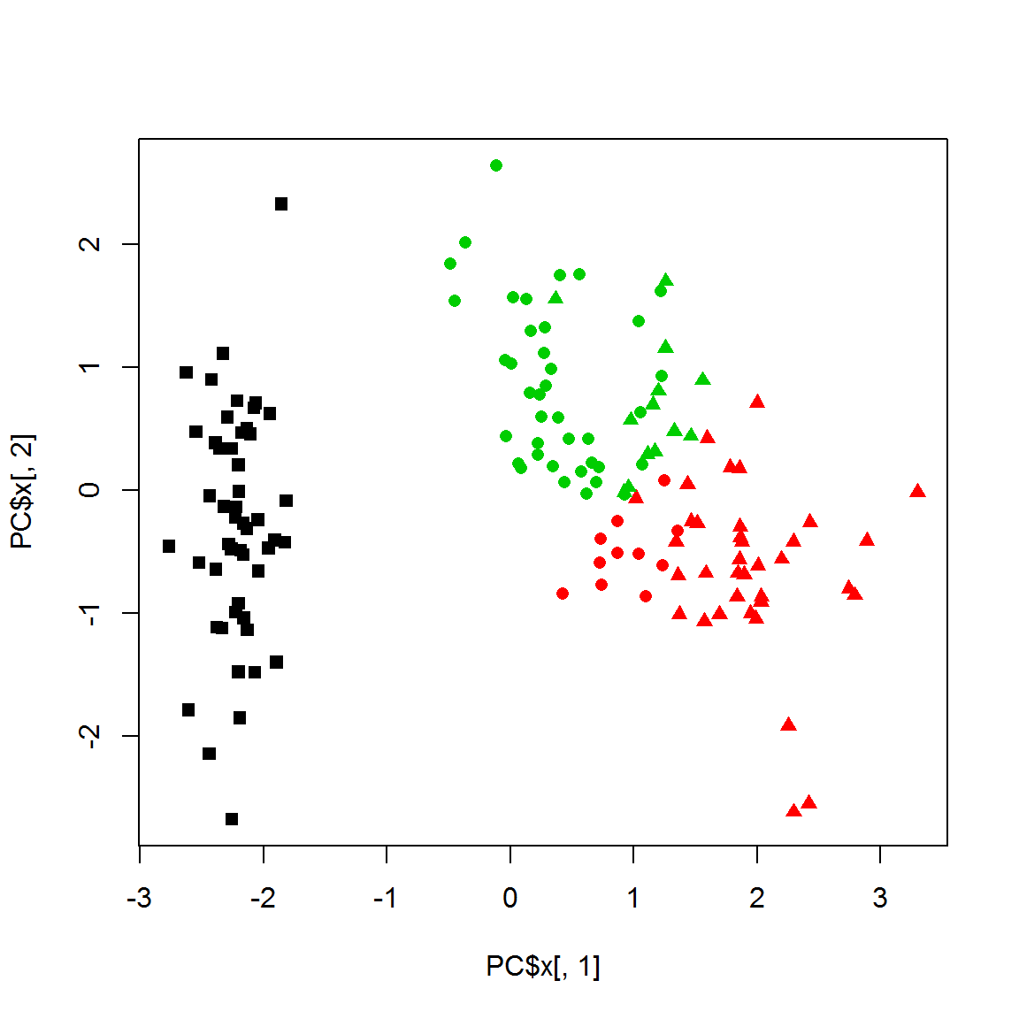
K-means is usually more stable to object removal than hierarchical methods.
cl1 = kmeans(X1,centers=3,nstart=10)$cluster
plot(PC$x[idx,1],PC$x[idx,2],col = cl1,pch=point1)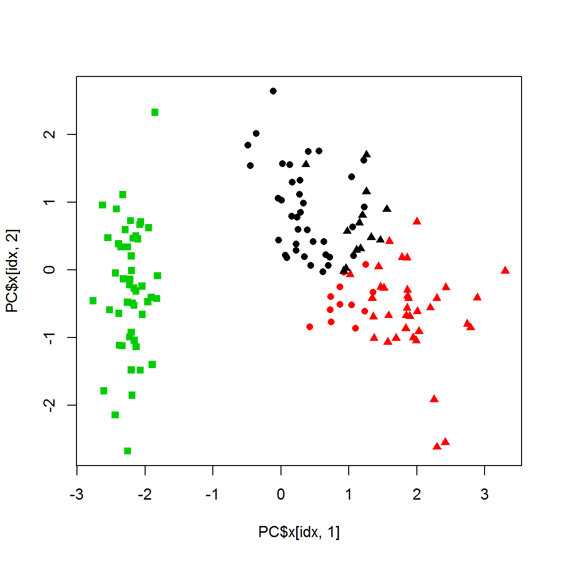
table(cl[idx],cl1)## cl1
## 1 2 3
## 1 0 0 49
## 2 0 46 0
## 3 51 1 01.3.2. Partitioning around medoids (PAM)
This method helps reducing effects of the outliers.
library(cluster)
cl = pam(X,k=3)$cluster
plot(PC$x[,1],PC$x[,2],col = cl,pch=point)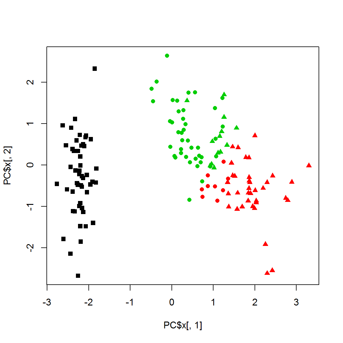
## stability to object removal ?
cl1 = pam(X1,k=3)$cluster
table(cl[idx],cl1)
## cl1
## 1 2 3
## 1 49 0 0
## 2 0 44 0
## 3 0 11 431.4. Optimal number of clusters
Unfortunately, there is no panacea. Try several methods and select the most reasonable and defendable result :)
You can look at within cluster variability (should be minimized):
wss=NULL

for (k in 1:10)
    wss[k] = kmeans(X,centers=k)$tot.withinss

plot(1:10,wss,lwd=2,type="b",pch=19,xlab="Number of clusters",ylab="Total Within-cluster SS",col=4,main="WSS vs number of clusters")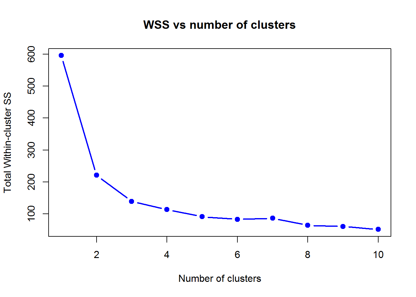
Here 2 or 3 clusters look reasonably good (at least much better than 1 cluster). Futher increase of clusters does not reduce WSS much.
You can use some specialized packages to make deeper investigation:
library(factoextra)## Warning: package 'factoextra' was built under R version 3.4.4## Loading required package: ggplot2## Welcome! Related Books: `Practical Guide To Cluster Analysis in R` at https://goo.gl/13EFCZlibrary(NbClust)
fviz_nbclust(X, kmeans, method = "silhouette")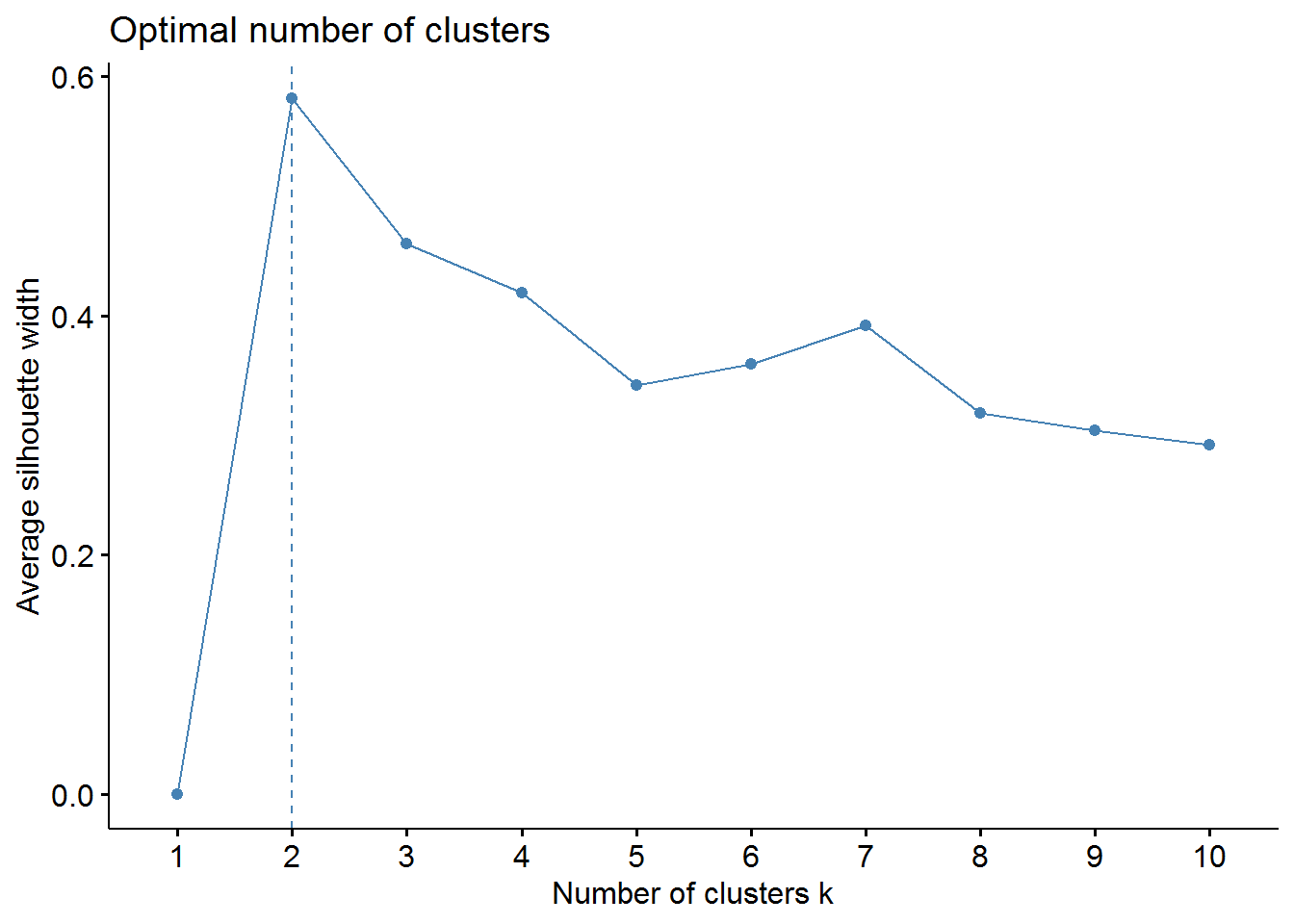
fviz_nbclust(X, kmeans, method = "wss")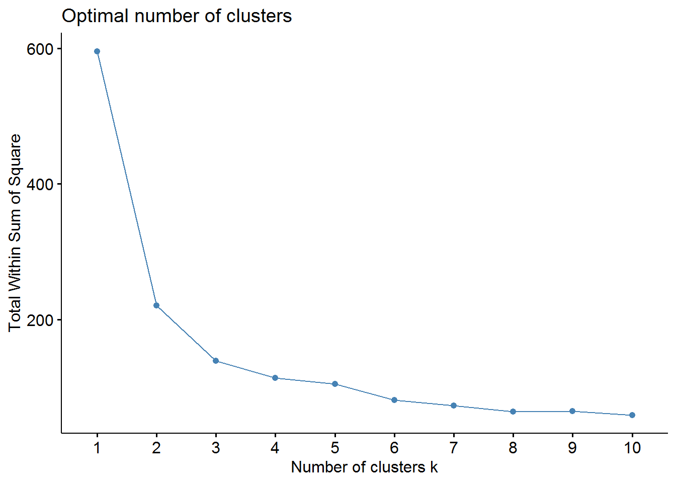
fviz_nbclust(X, kmeans, method = "gap_stat")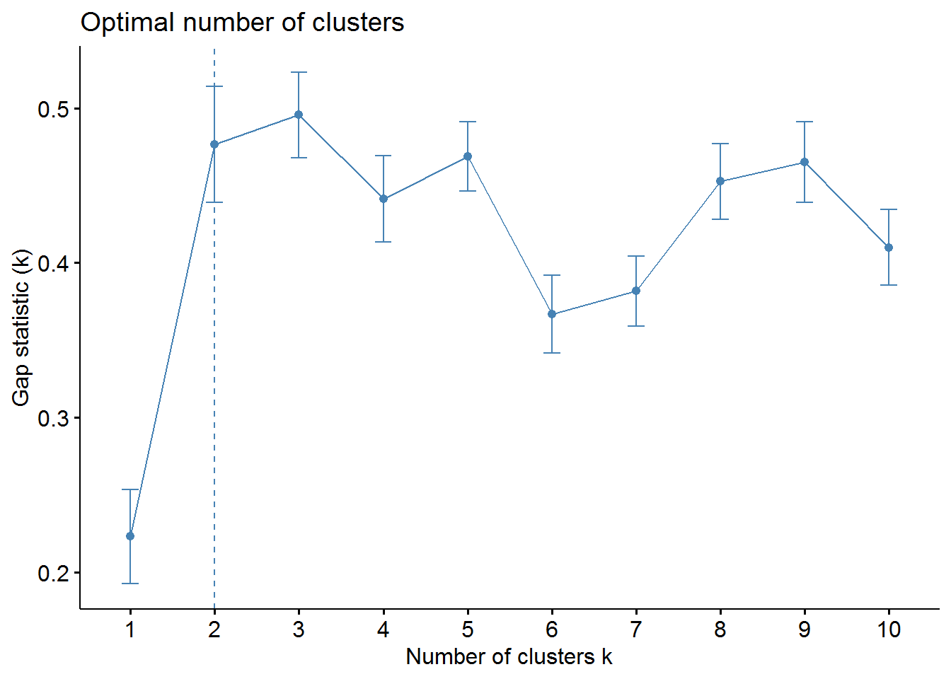
1.5. Density-based clustering
Density-based clustering allows extracting continuous clusters of complex shapes, that are not detected by standard distance-based methods. In bioinformatics, it is often used to determine the groups of cells in cytometry or single-cell genomics. The main parameter is epsilon - the radius of the “neighboring area”.
library(dbscan)## Warning: package 'dbscan' was built under R version 3.4.4res = dbscan(X,eps=0.5,minPts=5)
res## DBSCAN clustering for 150 objects.
## Parameters: eps = 0.5, minPts = 5
## The clustering contains 2 cluster(s) and 34 noise points.
##
## 0 1 2
## 34 45 71
##
## Available fields: cluster, eps, minPtsplot(PC$x[,1],PC$x[,2],col = 1+res$cluster,pch=point)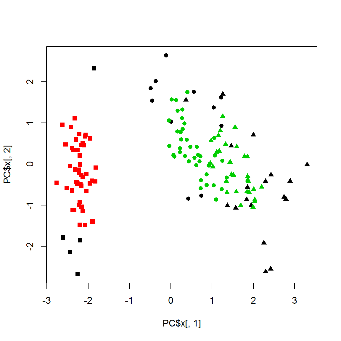
res = dbscan(X,eps=1.5,minPts=5)
plot(PC$x[,1],PC$x[,2],col = 1+res$cluster,pch=point)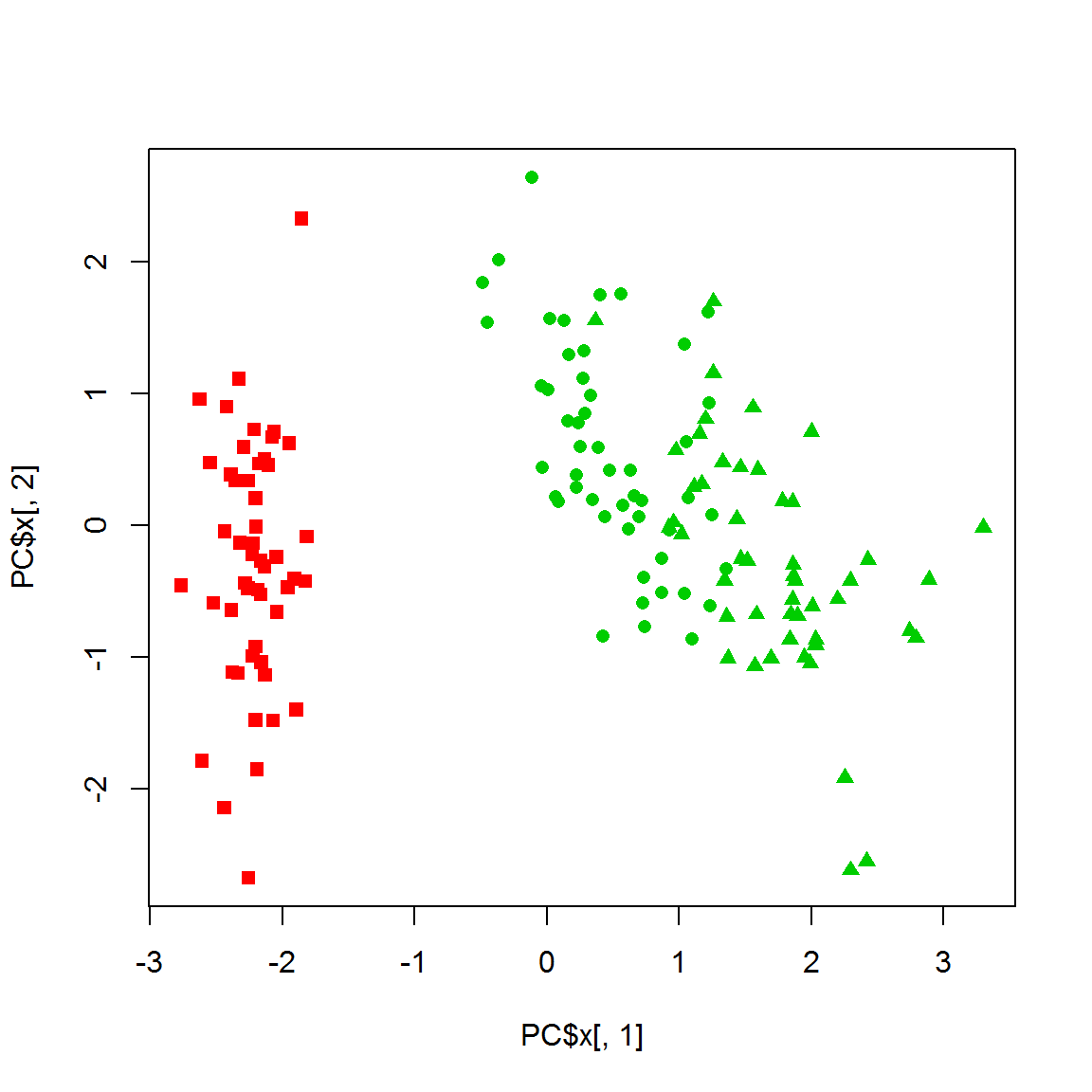
![]()